标签:
# 婚外情数据集
data(Affairs, package = "AER")
summary(Affairs)
table(Affairs$affairs)

# 用二值变量,是或否
Affairs$ynaffair[Affairs$affairs > 0] <- 1
Affairs$ynaffair[Affairs$affairs == 0] <- 0
Affairs$ynaffair <- factor(Affairs$ynaffair, levels = c(0, 1), labels = c("No", "Yes"))
table(Affairs$ynaffair)

#用glm
fit.full <- glm(ynaffair ~ gender + age + yearsmarried + children + religiousness + education + occupation + rating, data = Affairs, family = binomial())
summary(fit.full)
Deviance Residuals:
Min 1Q Median 3Q Max
-1.5713 -0.7499 -0.5690 -0.2539 2.5191
Coefficients:
Estimate Std. Error z value Pr(>|z|)
(Intercept) 1.37726 0.88776 1.551 0.120807
gendermale 0.28029 0.23909 1.172 0.241083
age -0.04426 0.01825 -2.425 0.015301 *
yearsmarried 0.09477 0.03221 2.942 0.003262 **
childrenyes 0.39767 0.29151 1.364 0.172508
religiousness -0.32472 0.08975 -3.618 0.000297 ***
education 0.02105 0.05051 0.417 0.676851
occupation 0.03092 0.07178 0.431 0.666630
rating -0.46845 0.09091 -5.153 2.56e-07 ***
---
Signif. codes: 0 ‘***’ 0.001 ‘**’ 0.01 ‘*’ 0.05 ‘.’ 0.1 ‘ ’ 1
(Dispersion parameter for binomial family taken to be 1)
Null deviance: 675.38 on 600 degrees of freedom
Residual deviance: 609.51 on 592 degrees of freedom
AIC: 627.51
Number of Fisher Scoring iterations: 4
#结果是有些变量不显著把它们都去掉
fit.reduced <- glm(ynaffair ~ age + yearsmarried +
religiousness + rating, data = Affairs, family = binomial())
summary(fit.reduced)
Call:
glm(formula = ynaffair ~ age + yearsmarried + religiousness +
rating, family = binomial(), data = Affairs)
Deviance Residuals:
Min 1Q Median 3Q Max
-1.6278 -0.7550 -0.5701 -0.2624 2.3998
Coefficients:
Estimate Std. Error z value Pr(>|z|)
(Intercept) 1.93083 0.61032 3.164 0.001558 **
age -0.03527 0.01736 -2.032 0.042127 *
yearsmarried 0.10062 0.02921 3.445 0.000571 ***
religiousness -0.32902 0.08945 -3.678 0.000235 ***
rating -0.46136 0.08884 -5.193 2.06e-07 ***
---
Signif. codes: 0 ‘***’ 0.001 ‘**’ 0.01 ‘*’ 0.05 ‘.’ 0.1 ‘ ’ 1
(Dispersion parameter for binomial family taken to be 1)
Null deviance: 675.38 on 600 degrees of freedom
Residual deviance: 615.36 on 596 degrees of freedom
AIC: 625.36
Number of Fisher Scoring iterations: 4
#如上,发现每个系数都非常显著。这是两模型嵌套,可以使用anova进行比较,对于广义线性回归,可用卡方检验。
anova(fit.reduced, fit.full, test = "Chisq")
Analysis of Deviance Table
Model 1: ynaffair ~ age + yearsmarried + religiousness + rating
Model 2: ynaffair ~ gender + age + yearsmarried + children + religiousness +
education + occupation + rating
Resid. Df Resid. Dev Df Deviance Pr(>Chi)
1 596 615.36
2 592 609.51 4 5.8474 0.2108
#卡方值不显著(0.21),表明新模型与包含了全部变量的模型拟合程度一样好。这可以确认添4个被去掉的变量不会显著提高方程的预测精度,可以依据更简单的模型进行解释。
13.2.1 解释模型参数
看回归系数:当其他预测变量不变时,一单位预测变量的变化可引起的响应变量对数优势比的变化。
coef(fit.reduced)
(Intercept) age yearsmarried religiousness rating
1.93083017 -0.03527112 0.10062274 -0.32902386 -0.46136144
由于对数优势比解释性差,可对结果进行指数化
exp(coef(fit.reduced))
(Intercept) age yearsmarried religiousness rating
6.8952321 0.9653437 1.1058594 0.7196258 0.6304248
可以看到婚龄增加一年,婚外情的优势比将乘以1.106(其他不变),年龄增加一岁,婚外情优势比乘以0.965。
因此,随着婚龄增加和年龄、宗教信仰与婚姻评分的降低,婚外情优势比将上升。
因为预测变量不能等于0,截距项在此处没有特定含义。
还可以使用confint函数获取置信区间。
exp(confint(fit.reduced))
Waiting for profiling to be done...
2.5 % 97.5 %
(Intercept) 2.1255764 23.3506030
age 0.9323342 0.9981470
yearsmarried 1.0448584 1.1718250
religiousness 0.6026782 0.8562807
rating 0.5286586 0.7493370
13.2.2 评价预测变量对结果概率的影响
testdata <- data.frame(rating = c(1, 2, 3, 4, 5),
    age = mean(Affairs$age), yearsmarried = mean(Affairs$yearsmarried),
    religiousness = mean(Affairs$religiousness))
testdata$prob <- predict(fit.reduced, newdata = testdata,
    type = "response")
testdata
rating age yearsmarried religiousness prob
1 1 32.48752 8.177696 3.116473 0.5302296
2 2 32.48752 8.177696 3.116473 0.4157377
3 3 32.48752 8.177696 3.116473 0.3096712
4 4 32.48752 8.177696 3.116473 0.2204547
5 5 32.48752 8.177696 3.116473 0.1513079
从结果看出,当婚姻评分从1(很不幸福)变成5(非常幸福),婚外情概率从0.53降低到0.15(假定年龄等因素不变),看看年龄影响
testdata <- data.frame(rating = mean(Affairs$rating),
    age = seq(17, 57, 10), yearsmarried = mean(Affairs$yearsmarried),
    religiousness = mean(Affairs$religiousness))
testdata$prob <- predict(fit.reduced, newdata = testdata,
    type = "response")
testdata
rating age yearsmarried religiousness prob
1 3.93178 17 8.177696 3.116473 0.3350834
2 3.93178 27 8.177696 3.116473 0.2615373
3 3.93178 37 8.177696 3.116473 0.1992953
4 3.93178 47 8.177696 3.116473 0.1488796
5 3.93178 57 8.177696 3.116473 0.1094738
从结果看出,当其他变量不变,年龄从17增加到57时,婚外情概率将从0.34降低到0.11,利用该方法,可探究每一个预测变量对结果概率的影响。
13.2.3 过度离势
过度离势:观测到的响应变量方差大于期望的二项分布的方式。这会导致奇异的标准误检验和不精确的显著性检验。
若出现过度离势,还可以用glm拟合Logistic回归,但此时需要将二项分布改为类二项分布。
检查方法:比较二项分布模型和残差偏差与残差自由度,如果比值比1大很多,便可认为存在过度离势。
本例中,比值=615.36/596=1.02,没有过度离势。
还可以对过度离势进行检验。为此,需要拟合模型两次,第一次使用family=binomial,第二次使用family=quasibinomial,假设第一次glm返回对象记为fit,第二次返回对象记为fit.od,用pchisq,提供的p值可对零假设(比值为1)与备择假设(比值不等于1)进行检验。
fit <- glm(ynaffair ~ age + yearsmarried + religiousness +
    rating, family = binomial(), data = Affairs)
fit.od <- glm(ynaffair ~ age + yearsmarried + religiousness +
    rating, family = quasibinomial(), data = Affairs)
pchisq(summary(fit.od)$dispersion * fit$df.residual,
    fit$df.residual, lower = F)
结果值为0.34不显著,因此不存在过度离势。
13.3 泊松回归
data(breslow.dat, package = "robust")
names(breslow.dat)
summary(breslow.dat[c(6, 7, 8, 10)])
opar <- par(no.readonly = TRUE)
par(mfrow = c(1, 2))
attach(breslow.dat)
hist(sumY, breaks = 20, xlab = "Seizure Count", main = "Distribution of Seizures")
boxplot(sumY ~ Trt, xlab = "Treatment", main = "Group Comparisons")
par(opar)
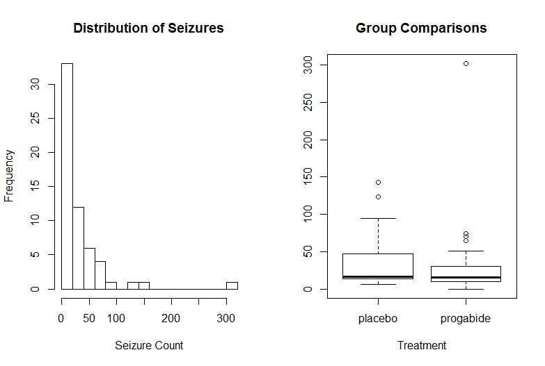
从图上可以看到因变量的偏倚特性及可能的离群点。药物治疗下发病数变小,方差也变小。与标准最小二乘回归不同,泊松回归并不关注方差异质量性。
fit <- glm(sumY ~ Base + Age + Trt, data = breslow.dat,
    family = poisson())
summary(fit)
结果非常显著
13.3.1 解释模型参数
coef(fit)
exp(coef(fit))
(Intercept) Base Age Trtprogabide
1.94882593 0.02265174 0.02274013 -0.15270095
年龄回归参数为0.0227,表明保持其他预测变量不变,年龄增加一岁,癫闲发病数的对数均值将增加0.03。
指数化系数中,年龄增加一岁,发病数乘以1.023。Trt变化,发病数*0.86。也就是说,保持发病数和年龄不变,服药组相对于安慰剂组发病数降低了20%。
13.3.2 过度离势
比值=559.44/55=10.17,大于1,说明存在过度离势。
也可以用以下方法检验过度离势。
library(qcc)
qcc.overdispersion.test(breslow.dat$sumY, type = "poisson")
P值为0,存在过度离势。
# fit model with quasipoisson
fit.od <- glm(sumY ~ Base + Age + Trt, data = breslow.dat,
family = quasipoisson())
summary(fit.od)
过度离势的原因:
1.遗漏了某个重要的预测变量
2.可能因为事件相关。泊松分布中,每个事件都被认为是独立发生的。就是对随便一位病人,每一次发病概率都认为是相互独立,但这并不成立。一个病人发生了40次病,第一次概率与第40次概率肯定不相同。
3.在纵向数据分析中,重复测量的数据由于内存群聚特性可导致过度离势。这里不讨论。
标签:
原文地址:http://www.cnblogs.com/MarsMercury/p/5019743.html