Machine Learning Review_Models(McCullah Pitts Model, Linear Networks, MLPBP)

标签：

McCullah Pitts Model

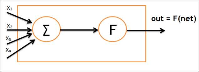
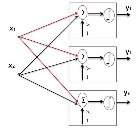
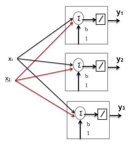
 Perceptron Model

Step:

1. initialise weight value

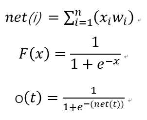
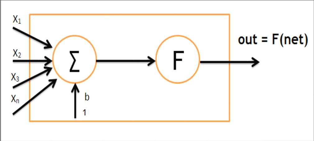
2. present input vector and obtain net input with 

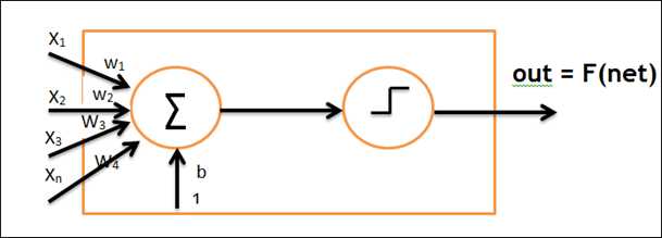
3. calculate output(with binary switch net > 0 or net <= 0)

4. update weight

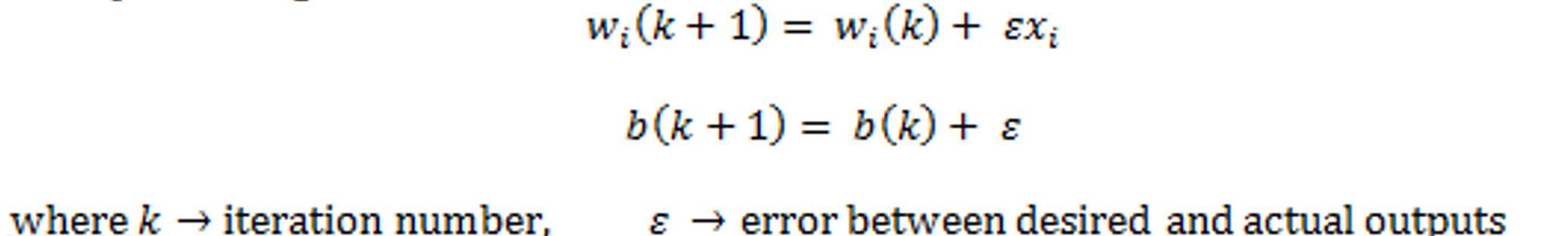
5. repeat uitil no change in weights or the maximum number of iterations is reached

6. repeat steps 2-4 for all training samples

Perceptron Model with Multiple Neurons

Step:

1. initialise weight value

2. present input vector and obtain net input with 

3. calculate output(with binary switch net > 0 or net <= 0)

4. update weight

5. repeat uitil no change in weights or the maximum number of iterations is reached

6. repeat steps 2-4 for all training samples

 Linear Networks – ADALINE

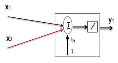
Transfer function is linear

Learns Least-Mean- Square Error (LMSE) or Delta Rule

Weights are updated to minimise MSE between y? and y

Input-output relationship must be linear

Step:

1. initialise weight value

2. present input vector and obtain net input with 

3. Change in weight

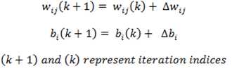
4. Update weights:

5. repeat steps 2-4 until  or the maximum number of iterations is reached

Pros: 

1. Easy to implement
2. Can generalise which is not the case with Perceptron

Cons:

Like the Perceptrons, it cannot train patterns belonging to non-linearly separable classes
Solution – cascaded ADALINE networks - MADALINE

MADALINE – Multiple ADALINE

 Single Layer Networks with Nonlinear Transfer Functions

Basis for Back Propagation networks

The sigmoid transfer function is a non-linear function and it has a simple derivative

Alogrithm:

1. initialise weight value

2. present input vector and obtain net input with 

3. Change in weight

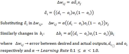
4. Update weights:

5. repeat steps 2-3 until no change in weights or the maximum number of iterations is reached

 Multi-Layer Perceptron (MLP) with Back Propagation (BP)

A MLP with BP is suitable for linearly separable inputs.

Generalising the Windrow-Hoff learning rule to ML networks and non-linear differential activation functions created the BP algorithm

Learning involves the presentation of input-output pairs, finding the mean squared error between desired and actual outputs, and adjusting the weights to reduce the difference

Learning uses a gradient descent search technique to minimise the cost function which is the MSE

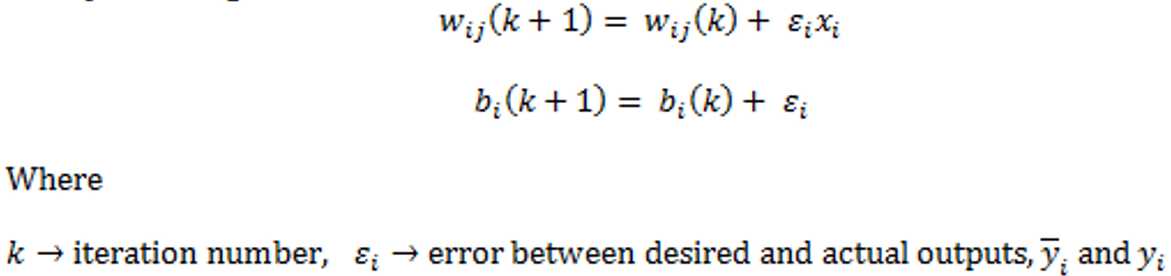
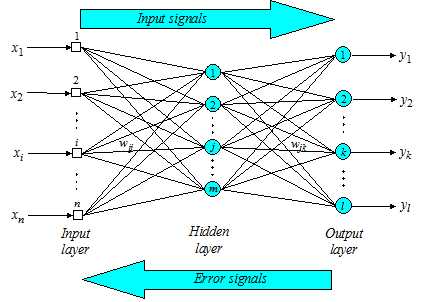
Algorithms:

1. initialise weight value

2. present input vector x1(p),x2(p).....xn(p) and desired outputs yd1(p) yd2(p) ..... ydn(p) and calculate actual output:

 where n is the number of inputs of neuron j in the hidden layer, and sigmod is the sigmod activation function.

3. weight training--- update the weights in the back-propagation network propagating backward the errors associated with output neurons.

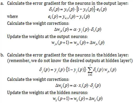
4. iteration - increase iteration p by one, go back to step 2 and repeat the process until the selected error criterion is satisfied.

Machine Learning Review_Models(McCullah Pitts Model, Linear Networks, MLPBP)

标签：

原文地址：http://www.cnblogs.com/eli-ayase/p/5899096.html