标签:data- max axis ogr info core ssis weight volume
Convolutional Neural Networks are made up of neurons that have learnable weights and biases. Each neuron receives some inputs, performs a dot product and optionally follows it with a non-linearity. They still have a loss function (e.g. SVM/Softmax) on the last (fully-connected) layer and all the tips/tricks we developed for learning regular Neural Networks still apply.
ConvNet architectures make the explicit assumption that the inputs are images, which allows us to encode certain properties into the architecture and reduce the amount of parameters in the network.
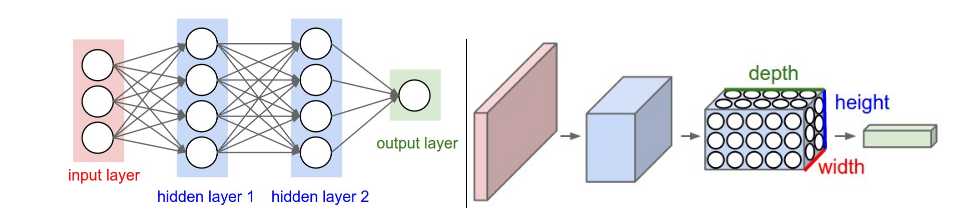
3D volumes of neurons:the layers of a ConvNet have neurons arranged in 3 dimensions: width, height, depth ( third dimension of an activation volume, not to the depth of a full Neural Network ).
the final output layer would for CIFAR-10 have dimensions 1x1x10, because by the end of the ConvNet architecture we will reduce the full image into a single vector of class scores, arranged along the depth dimension. Here is a visualization:
Three main types of layers to build ConvNet architectures: Convolutional Layer, Pooling Layer, and Fully-Connected Layer (exactly as seen in regular Neural Networks).
Example Architecture: a simple ConvNet for CIFAR-10 classification could have the architecture [INPUT - CONV - RELU - POOL - FC]. In more detail:
The CONV/FC layers perform transformations that are a function of the activations in the input volume and the parameters (the weights and biases of the neurons).
The parameters in the CONV/FC layers will be trained with gradient descent
The RELU/POOL layers will implement a fixed function
The connections are local in space (along width and height), but always full along the entire depth of the input volume.
Example 1. For example, input volume has size [32x32x3], If the receptive field (or the filter size) is 5x5, then each neuron in the Conv Layer will have weights to a [5x5x3] region in the input volume, for a total of 5*5*3 = 75 weights (and +1 bias parameter). Notice that the extent of the connectivity along the depth axis must be 3, since this is the depth of the input volume.
Example 2. Suppose an input volume had size [16x16x20]. Then using an example receptive field size of 3x3, every neuron in the Conv Layer would now have a total of 3*3*20 = 180 connections to the input volume. Notice that, again, the connectivity is local in space (e.g. 3x3), but full along the input depth (20).
Three hyperparameters:depth, stride and zero-padding.
depth:number of filters we would like to use
input volume size in one dimension (W), the receptive field size of the Conv Layer neurons (F), the stride size (S), and the amount of zero padding used (P)
output size: (W?F+2P)/S+1
Summary
A common setting of the hyperparameters is F=3,S=1,P=1F=3,S=1,P=1.
Its function is to progressively reduce the spatial size of the representation to reduce the amount of parameters and computation in the network, and hence to also control overfitting.
The Pooling Layer operates independently on every depth slice of the input and resizes it spatially, using the MAX operation.
The most common form is a pooling layer with filters of size 2x2 applied with a stride of 2 downsamples every depth slice in the input by 2 along both width and height, discarding 75% of the activations.
Neurons in a fully connected layer have full connections to all activations in the previous layer, as seen in regular Neural Networks. Their activations can hence be computed with a matrix multiplication followed by a bias offset.
the most common ConvNet architecture follows the pattern:
INPUT -> [[CONV -> RELU]*N -> POOL?]*M -> [FC -> RELU]*K -> FC
for example
INPUT -> [CONV -> RELU -> CONV -> RELU -> POOL]*3 -> [FC -> RELU]*2 -> FC Here we see two CONV layers stacked before every POOL layer. This is generally a good idea for larger and deeper networks, because multiple stacked CONV layers can develop more complex features of the input volume before the destructive pooling operation.Prefer a stack of small filter CONV to one large receptive field CONV layer.
Suppose that you stack three 3x3 CONV layers on top of each other (with non-linearities in between, of course). In this arrangement, each neuron on the first CONV layer has a 3x3 view of the input volume. A neuron on the second CONV layer has a 3x3 view of the first CONV layer, and hence by extension a 5x5 view of the input volume. Similarly, a neuron on the third CONV layer has a 3x3 view of the 2nd CONV layer, and hence a 7x7 view of the input volume. Suppose that instead of these three layers of 3x3 CONV, we only wanted to use a single CONV layer with 7x7 receptive fields. These neurons would have a receptive field size of the input volume that is identical in spatial extent (7x7), but with several disadvantages. First, the neurons would be computing a linear function over the input, while the three stacks of CONV layers contain non-linearities that make their features more expressive. Second, if we suppose that all the volumes have CC channels, then it can be seen that the single 7x7 CONV layer would contain C×(7×7×C)=49C^2 parameters, while the three 3x3 CONV layers would only contain 3×(C×(3×3×C))=27C^2 parameters. Intuitively, stacking CONV layers with tiny filters as opposed to having one CONV layer with big filters allows us to express more powerful features of the input, and with fewer parameters. As a practical disadvantage, we might need more memory to hold all the intermediate CONV layer results if we plan to do backpropagation.
The input layer (that contains the image) should be divisible by 2 many times. Common numbers include 32 (e.g. CIFAR-10), 64, 96 (e.g. STL-10), or 224 (e.g. common ImageNet ConvNets), 384, and 512.
The conv layers should be using small filters (e.g. 3x3 or at most 5x5), using a stride of S=1S=1, and crucially, padding the input volume with zeros in such way that the conv layer does not alter the spatial dimensions of the input.
For a general F, it can be seen that P=(F?1)/2 preserves the input size. If you must use bigger filter sizes (such as 7x7 or so), it is only common to see this on the very first conv layer that is looking at the input image.
The pool layers are in charge of downsampling the spatial dimensions of the input. The most common setting is to use max-pooling with 2x2 receptive fields (i.e. F=2F=2), and with a stride of 2 (i.e. S=2S=2)
Why use stride of 1 in CONV?
Smaller strides work better in practice. Additionally, as already mentioned stride 1 allows us to leave all spatial down-sampling to the POOL layers, with the CONV layers only transforming the input volume depth-wise.
Why use padding?
In addition to the aforementioned benefit of keeping the spatial sizes constant after CONV, doing this actually improves performance. If the CONV layers were to not zero-pad the inputs and only perform valid convolutions, then the size of the volumes would reduce by a small amount after each CONV, and the information at the borders would be “washed away” too quickly.
In practice, very few people train an entire Convolutional Network from scratch (with random initialization), because it is relatively rare to have a dataset of sufficient size. Instead, it is common to pretrain a ConvNet on a very large dataset (e.g. ImageNet, which contains 1.2 million images with 1000 categories), and then use the ConvNet either as an initialization or a fixed feature extractor for the task of interest. The three major Transfer Learning scenarios look as follows:
When and how to fine-tune? How do you decide what type of transfer learning you should perform on a new dataset? This is a function of several factors, but the two most important ones are the size of the new dataset (small or big), and its similarity to the original dataset (e.g. ImageNet-like in terms of the content of images and the classes, or very different, such as microscope images). Keeping in mind that ConvNet features are more generic in early layers and more original-dataset-specific in later layers, here are some common rules of thumb for navigating the 4 major scenarios:
Practical advice. There are a few additional things to keep in mind when performing Transfer Learning:
Convolutional Neural Networks (CNNs / ConvNets) Notes
标签:data- max axis ogr info core ssis weight volume
原文地址:http://www.cnblogs.com/rfliu0/p/6293064.html