标签:.com ons length problem included within ack computer alt
Anomaly detection
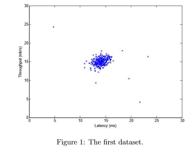
In this exercise, you will implement an anomaly detection algorithm to detect anomalous behavior in server computers. The features measure the throughput (mb/s) and latency (ms) of response of each server. While your servers were operating, you collected m = 307 examples of how they were behaving, and thus have an unlabeled dataset {x(1),...,x(m)}. You suspect that the vast majority of these examples are “normal” (non-anomalous) examples of the servers operating normally, but there might also be some examples of servers acting anomalously within this dataset.
You will use a Gaussian model to detect anomalous examples in your dataset. You will ?rst start on a 2D dataset that will allow you to visualize what the algorithm is doing. On that dataset you will ?t a Gaussian distribution and then ?nd values that have very low probability and hence can be considered anomalies. After that, you will apply the anomaly detection algorithm to a larger dataset with many dimensions. You will be using ex8.m for this part of the exercise.
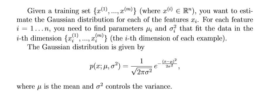
Gaussian distribution
To perform anomaly detection, you will ?rst need to ?t a model to the data’s distribution.
Estimating parameters for a Gaussian
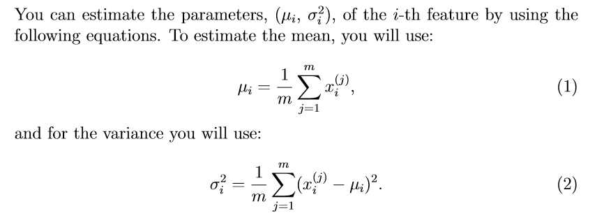
Your task is to complete the code in estimateGaussian.m. This function takes as input the data matrix X and should output an n-dimension vector mu that holds the mean of all the n features and another n-dimension vector sigma2 that holds the variances of all the features. You can implement this using a for-loop over every feature and every training example (though a vectorized implementation might be more e?cient; feel free to use a vectorized implementation if you prefer). Note that in Octave/MATLAB, the var function will (by default) use m?1 , instead of m, when computing σ2.
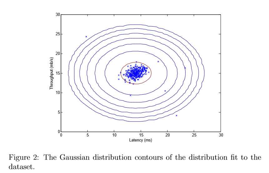
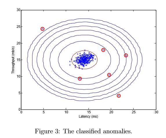
From your plot, you can see that most of the examples are in the region with the highest probability, while the anomalous examples are in the regions with lower probabilities.
function [mu sigma2] = estimateGaussian(X)

[m, n] = size(X);

mu = zeros(n, 1);
sigma2 = zeros(n, 1);

mu = (mean(X))‘;
sigma2 = (var(X))‘*(m-1)/m;


end
%  Estimate my and sigma2
[mu sigma2] = estimateGaussian(X);

%  Returns the density of the multivariate normal at each data point (row)
%  of X
p = multivariateGaussian(X, mu, sigma2);
Now that you have estimated the Gaussian parameters, you can investigate which examples have a very high probability given this distribution and which examples have a very low probability. The low probability examples are more likely to be the anomalies in our dataset. One way to determine which examples are anomalies is to select a threshold based on a cross validation set. In this part of the exercise, you will implement an algorithm to select the threshold ε using the F1 score on a cross validation set.
In the provided code selectThreshold.m, there is already a loop that will try many di?erent values of ε and select the best ε based on the F1 score.
function [bestEpsilon bestF1] = selectThreshold(yval, pval)

bestEpsilon = 0;
bestF1 = 0;
F1 = 0;

stepsize = (max(pval) - min(pval)) / 1000;
for epsilon = min(pval):stepsize:max(pval)

cvPredictions = pval<epsilon;
tp = sum((cvPredictions == 1)&(yval == 1)); %true positives
fp = sum((cvPredictions == 1)&(yval == 0));
fn = sum((cvPredictions == 0)&(yval == 1));

prec = tp/(tp+fp+1e-10);
rec = tp/(tp+fn+1e-10);
F1 = 2*prec*rec/(prec+rec+1e-10);

    if F1 > bestF1
       bestF1 = F1;
       bestEpsilon = epsilon;
    end
end

end
%  Loads the second dataset. You should now have the
%  variables X, Xval, yval in your environment
load(‘ex8data2.mat‘);

%  Apply the same steps to the larger dataset
[mu sigma2] = estimateGaussian(X);

%  Training set
p = multivariateGaussian(X, mu, sigma2);

%  Cross-validation set
pval = multivariateGaussian(Xval, mu, sigma2);

%  Find the best threshold
[epsilon F1] = selectThreshold(yval, pval);

fprintf(‘Best epsilon found using cross-validation: %e\n‘, epsilon);
fprintf(‘Best F1 on Cross Validation Set:  %f\n‘, F1);
fprintf(‘# Outliers found: %d\n‘, sum(p < epsilon));
Recommender Systems
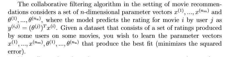
In this part of the exercise, you will implement the collaborative ?ltering learning algorithm and apply it to a dataset of movie ratings.2 This dataset consists of ratings on a scale of 1 to 5. The dataset has nu = 943 users, and nm = 1682 movies.
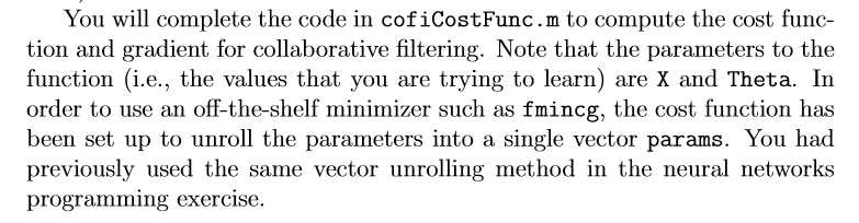
In the next parts of this exercise, you will implement the function cofiCostFunc.m that computes the collaborative ?tlering objective function and gradient. After implementing the cost function and gradient, you will use fmincg.m to learn the parameters for collaborative ?ltering.
Movie ratings dataset
The ?rst part of the script ex8 cofi.m will load the dataset ex8 movies.mat, providing the variables Y and R in your Octave/MATLAB environment.
The matrix Y (a num movies×num users matrix) stores the ratings y(i,j) (from 1 to 5). The matrix R is an binary-valued indicator matrix, where R(i,j) = 1 if user j gave a rating to movie i, and R(i,j) = 0 otherwise. The objective of collaborative ?ltering is to predict movie ratings for the movies that users have not yet rated, that is, the entries with R(i,j) = 0. This will allow us to recommend the movies with the highest predicted ratings to the user.
To help you understand the matrix Y, the script ex8 cofi.m will compute the average movie rating for the ?rst movie (Toy Story) and output the average rating to the screen.
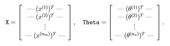
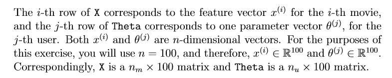
Throughout this part of the exercise, you will also be working with the matrices, X and Theta:
Collaborative ?ltering learning algorith
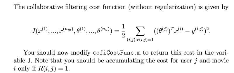
Now, you will start implementing the collaborative ?ltering learning algorithm. You will start by implementing the cost function (without regularization).
Collaborative ?ltering cost function
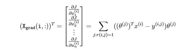
Collaborative ?ltering gradient
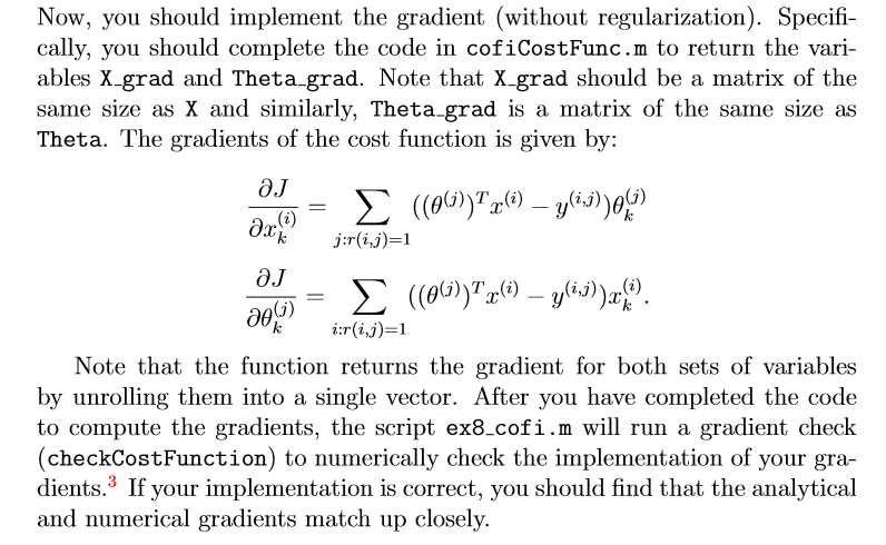
(one for looping over movies to compute ?J/?x(i) k for each movie, and one for looping over users to compute ?J/?θ(j) k for each user).
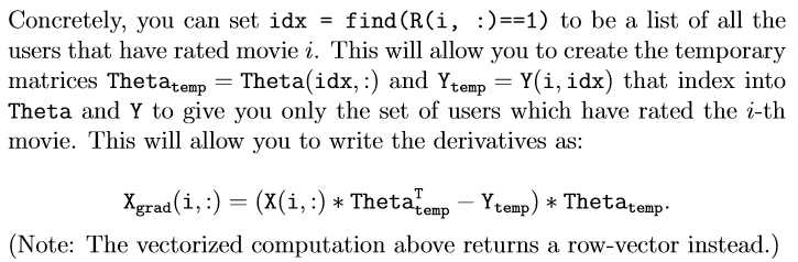
Intuitively, when you consider the features for the i-th movie, you only need to be concern about the users who had given ratings to the movie, and this allows you to remove all the other users from Theta and Y.
Regularized cost function
The cost function for collaborative ?ltering with regularization is given by
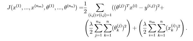
function [J, grad] = cofiCostFunc(params, Y, R, num_users, num_movies, ...
                                  num_features, lambda)
%COFICOSTFUNC Collaborative filtering cost function
%   [J, grad] = COFICOSTFUNC(params, Y, R, num_users, num_movies, ...
%   num_features, lambda) returns the cost and gradient for the
%   collaborative filtering problem.
%

% Unfold the U and W matrices from params
X = reshape(params(1:num_movies*num_features), num_movies, num_features);
Theta = reshape(params(num_movies*num_features+1:end), ...
                num_users, num_features);


% You need to return the following values correctly
J = 0;
X_grad = zeros(size(X));
Theta_grad = zeros(size(Theta));

% ====================== YOUR CODE HERE ======================
% Instructions: Compute the cost function and gradient for collaborative
%               filtering. Concretely, you should first implement the cost
%               function (without regularization) and make sure it is
%               matches our costs. After that, you should implement the
%               gradient and use the checkCostFunction routine to check
%               that the gradient is correct. Finally, you should implement
%               regularization.
%
% Notes: X - num_movies  x num_features matrix of movie features
%        Theta - num_users  x num_features matrix of user features
%        Y - num_movies x num_users matrix of user ratings of movies
%        R - num_movies x num_users matrix, where R(i, j) = 1 if the
%            i-th movie was rated by the j-th user
%
% You should set the following variables correctly:
%
%        X_grad - num_movies x num_features matrix, containing the
%                 partial derivatives w.r.t. to each element of X
%        Theta_grad - num_users x num_features matrix, containing the
%                     partial derivatives w.r.t. to each element of Theta
%

H =X*Theta‘;
J = 0.5*sum(sum(R.*(H-Y).^2))+0.5*lambda*sum(sum(Theta.^2))+0.5*lambda*sum(sum(X.^2));

X_grad = R.*(H-Y)*Theta + lambda*X;
Theta_grad = (R.*(H-Y))‘*X + lambda*Theta;

% =============================================================

grad = [X_grad(:); Theta_grad(:)];

end
%% Machine Learning Online Class
%  Exercise 8 | Anomaly Detection and Collaborative Filtering
%
%  Instructions
%  ------------
%
%  This file contains code that helps you get started on the
%  exercise. You will need to complete the following functions:
%
%     estimateGaussian.m
%     selectThreshold.m
%     cofiCostFunc.m
%
%  For this exercise, you will not need to change any code in this file,
%  or any other files other than those mentioned above.
%

%% =============== Part 1: Loading movie ratings dataset ================
%  You will start by loading the movie ratings dataset to understand the
%  structure of the data.
%
fprintf(‘Loading movie ratings dataset.\n\n‘);

%  Load data
load (‘ex8_movies.mat‘);

%  Y is a 1682x943 matrix, containing ratings (1-5) of 1682 movies on
%  943 users
%
%  R is a 1682x943 matrix, where R(i,j) = 1 if and only if user j gave a
%  rating to movie i

%  From the matrix, we can compute statistics like average rating.
fprintf(‘Average rating for movie 1 (Toy Story): %f / 5\n\n‘, ...
        mean(Y(1, R(1, :))));

%  We can "visualize" the ratings matrix by plotting it with imagesc
imagesc(Y);
ylabel(‘Movies‘);
xlabel(‘Users‘);

fprintf(‘\nProgram paused. Press enter to continue.\n‘);
pause;

%% ============ Part 2: Collaborative Filtering Cost Function ===========
%  You will now implement the cost function for collaborative filtering.
%  To help you debug your cost function, we have included set of weights
%  that we trained on that. Specifically, you should complete the code in
%  cofiCostFunc.m to return J.

%  Load pre-trained weights (X, Theta, num_users, num_movies, num_features)
load (‘ex8_movieParams.mat‘);

%  Reduce the data set size so that this runs faster
num_users = 4; num_movies = 5; num_features = 3;
X = X(1:num_movies, 1:num_features);
Theta = Theta(1:num_users, 1:num_features);
Y = Y(1:num_movies, 1:num_users);
R = R(1:num_movies, 1:num_users);

%  Evaluate cost function
J = cofiCostFunc([X(:) ; Theta(:)], Y, R, num_users, num_movies, ...
               num_features, 0);

fprintf([‘Cost at loaded parameters: %f ‘...
         ‘\n(this value should be about 22.22)\n‘], J);

fprintf(‘\nProgram paused. Press enter to continue.\n‘);
pause;


%% ============== Part 3: Collaborative Filtering Gradient ==============
%  Once your cost function matches up with ours, you should now implement
%  the collaborative filtering gradient function. Specifically, you should
%  complete the code in cofiCostFunc.m to return the grad argument.
%
fprintf(‘\nChecking Gradients (without regularization) ... \n‘);

%  Check gradients by running checkNNGradients
checkCostFunction;

fprintf(‘\nProgram paused. Press enter to continue.\n‘);
pause;


%% ========= Part 4: Collaborative Filtering Cost Regularization ========
%  Now, you should implement regularization for the cost function for
%  collaborative filtering. You can implement it by adding the cost of
%  regularization to the original cost computation.
%

%  Evaluate cost function
J = cofiCostFunc([X(:) ; Theta(:)], Y, R, num_users, num_movies, ...
               num_features, 1.5);

fprintf([‘Cost at loaded parameters (lambda = 1.5): %f ‘...
         ‘\n(this value should be about 31.34)\n‘], J);

fprintf(‘\nProgram paused. Press enter to continue.\n‘);
pause;


%% ======= Part 5: Collaborative Filtering Gradient Regularization ======
%  Once your cost matches up with ours, you should proceed to implement
%  regularization for the gradient.
%

%
fprintf(‘\nChecking Gradients (with regularization) ... \n‘);

%  Check gradients by running checkNNGradients
checkCostFunction(1.5);

fprintf(‘\nProgram paused. Press enter to continue.\n‘);
pause;


%% ============== Part 6: Entering ratings for a new user ===============
%  Before we will train the collaborative filtering model, we will first
%  add ratings that correspond to a new user that we just observed. This
%  part of the code will also allow you to put in your own ratings for the
%  movies in our dataset!
%
movieList = loadMovieList();

%  Initialize my ratings
my_ratings = zeros(1682, 1);

% Check the file movie_idx.txt for id of each movie in our dataset
% For example, Toy Story (1995) has ID 1, so to rate it "4", you can set
my_ratings(1) = 4;

% Or suppose did not enjoy Silence of the Lambs (1991), you can set
my_ratings(98) = 2;

% We have selected a few movies we liked / did not like and the ratings we
% gave are as follows:
my_ratings(7) = 3;
my_ratings(12)= 5;
my_ratings(54) = 4;
my_ratings(64)= 5;
my_ratings(66)= 3;
my_ratings(69) = 5;
my_ratings(183) = 4;
my_ratings(226) = 5;
my_ratings(355)= 5;

fprintf(‘\n\nNew user ratings:\n‘);
for i = 1:length(my_ratings)
    if my_ratings(i) > 0
        fprintf(‘Rated %d for %s\n‘, my_ratings(i), ...
                 movieList{i});
    end
end

fprintf(‘\nProgram paused. Press enter to continue.\n‘);
pause;


%% ================== Part 7: Learning Movie Ratings ====================
%  Now, you will train the collaborative filtering model on a movie rating
%  dataset of 1682 movies and 943 users
%

fprintf(‘\nTraining collaborative filtering...\n‘);

%  Load data
load(‘ex8_movies.mat‘);

%  Y is a 1682x943 matrix, containing ratings (1-5) of 1682 movies by
%  943 users
%
%  R is a 1682x943 matrix, where R(i,j) = 1 if and only if user j gave a
%  rating to movie i

%  Add our own ratings to the data matrix
Y = [my_ratings Y];
R = [(my_ratings ~= 0) R];

%  Normalize Ratings
[Ynorm, Ymean] = normalizeRatings(Y, R);

%  Useful Values
num_users = size(Y, 2);
num_movies = size(Y, 1);
num_features = 10;

% Set Initial Parameters (Theta, X)
X = randn(num_movies, num_features);
Theta = randn(num_users, num_features);

initial_parameters = [X(:); Theta(:)];

% Set options for fmincg
options = optimset(‘GradObj‘, ‘on‘, ‘MaxIter‘, 100);

% Set Regularization
lambda = 10;
theta = fmincg (@(t)(cofiCostFunc(t, Ynorm, R, num_users, num_movies, ...
                                num_features, lambda)), ...
                initial_parameters, options);

% Unfold the returned theta back into U and W
X = reshape(theta(1:num_movies*num_features), num_movies, num_features);
Theta = reshape(theta(num_movies*num_features+1:end), ...
                num_users, num_features);

fprintf(‘Recommender system learning completed.\n‘);

fprintf(‘\nProgram paused. Press enter to continue.\n‘);
pause;

%% ================== Part 8: Recommendation for you ====================
%  After training the model, you can now make recommendations by computing
%  the predictions matrix.
%

p = X * Theta‘;
my_predictions = p(:,1) + Ymean;

movieList = loadMovieList();

[r, ix] = sort(my_predictions, ‘descend‘);
fprintf(‘\nTop recommendations for you:\n‘);
for i=1:10
    j = ix(i);
    fprintf(‘Predicting rating %.1f for movie %s\n‘, my_predictions(j), ...
            movieList{j});
end

fprintf(‘\n\nOriginal ratings provided:\n‘);
for i = 1:length(my_ratings)
    if my_ratings(i) > 0
        fprintf(‘Rated %d for %s\n‘, my_ratings(i), ...
                 movieList{i});
    end
end
coursera:machine learing--code-6
标签:.com ons length problem included within ack computer alt
原文地址:http://www.cnblogs.com/kprac/p/6389292.html