标签:数值 http plot 索引 脚本 互联网公司 com 对比 大小
有意思的是,scipy囊括了numpy的命名空间,也就是说所有np.func都可以通过sp.func等价调用。
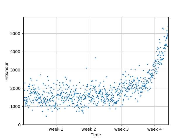
本部分对一个互联网公司的流量进行拟合处理,学习最基本的机器学习应用。
import os
import scipy as sp
import matplotlib.pyplot as plt

data_dir = os.path.join(
    os.path.dirname(os.path.realpath(__file__)), "..", "data")
# __file__ 是用来获得模块所在的路径的,这可能得到的是一个相对路径,
# os.path.dirname(__file__) ,相对路径时返回值为空,
# 为了得到绝对路径,需要 os.path.dirname(os.path.realpath(__file__))。
# .realpath得到完整路径加文件名
# .dirname会去掉脚本名,只保留路径
# print(os.path.realpath(__file__))
# print(os.path.dirname(os.path.realpath(__file__)))
这里没有采用原书的读取方式,似乎原作者不知道这样写更为简洁:
# data = sp.genfromtxt(os.path.join(data_dir, "web_traffic.tsv"), delimiter="\t")
# x = data[:,0]
# y = data[:,1]

# 和上面三行等价
x,y = sp.loadtxt(os.path.join(data_dir, "web_traffic.tsv"), delimiter="\t",unpack=True)

print("非法数据:", sp.sum(sp.isnan(y)))    # 统计nan缺失
x = x[~sp.isnan(y)]                        # 布尔索引
y = y[~sp.isnan(y)]                        # 布尔索引
这个函数写的很精妙,有不少使用了python高级技巧的地方,值得学习:
list+zip的运用,list生成器的运用等等
顺便一提,sp.poly1d()生成对象有属性f.order,可以查看自身的阶数。
colors = [‘g‘, ‘k‘, ‘b‘, ‘m‘, ‘r‘] #<-----------
linestyles = [‘-‘, ‘-.‘, ‘--‘, ‘:‘, ‘-‘] #<-----------

def plot_models(x, y, models, fname, mx=None, ymax=None, xmin=None):
    ‘‘‘
    绘制原数据散点图和拟合线图
    :param x:        横坐标
    :param y:        纵坐标
    :param models:   拟合线(list传入)
    :param fname:    保存图像名
    :param mx:       拟合线x的list是否给定了
    :param ymax:     y轴上限
    :param xmin:     x轴下限
    :return:         None
    ‘‘‘
    plt.clf()                                                         # 清空当前坐标上图像
    plt.scatter(x, y, s=10, alpha=1, marker=‘.‘)
    # c:散点的颜色
    # s:散点的大小
    # alpha:是透明程度
    # plt.title("上个月网络流量图")
    plt.xlabel("Time")
    plt.ylabel("Hits/hour")
    plt.xticks(
        [w*7*24 for w in range(10)], ["week %i" % w for w in range(10)])

    if models:                                                       # 是不是绘制拟合线
        if mx is None:
            mx = sp.linspace(0, x[-1], 1000)
        for model, style, color in zip(models, linestyles, colors): #<-----------
            plt.plot(mx, model(mx), linestyle=style, linewidth=2, c=color) #<-----------

        plt.legend(["d=%i" % m.order for m in models], loc="upper left") #<-----------
    plt.autoscale(tight=True)
    plt.ylim(ymin=0)
    if ymax:
        plt.ylim(ymax=ymax)
    if xmin:
        plt.xlim(xmin=xmin)
    plt.grid(True, linestyle=‘-‘, color=‘0.75‘) #<-----------        # 网格线设置,color应该是灰度
    plt.savefig(fname)
# 绘制原始数据散点图
plot_models(x, y, None, os.path.join( "..", "1400_01_01.png"))
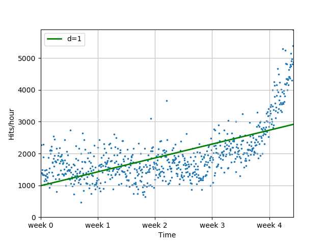
fp1, res, rank, sv, rcond = sp.polyfit(x, y, 1, full=True)
print("拟合参数: %s" % fp1)
print("误差数值: %s" % res)
f1 = sp.poly1d(fp1)
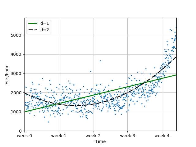
f2 = sp.poly1d(sp.polyfit(x, y, 2))
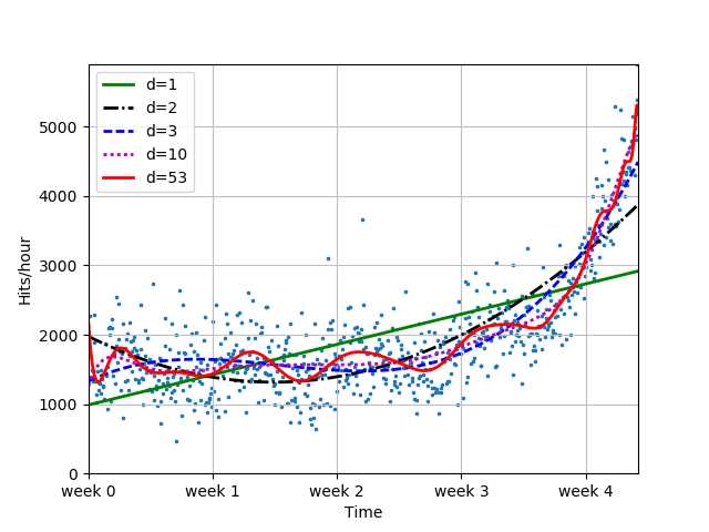
f3 = sp.poly1d(sp.polyfit(x, y, 3))
f10 = sp.poly1d(sp.polyfit(x, y, 10))
f100 = sp.poly1d(sp.polyfit(x, y, 100))
plot_models(x, y, [f1], os.path.join("..", "1400_01_02.png"))
plot_models(x, y, [f1, f2], os.path.join("..", "1400_01_03.png"))
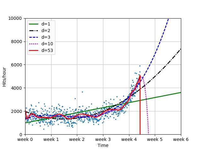
plot_models(x, y, [f1, f2, f3, f10, f100], os.path.join("..", "1400_01_04.png"))
分离转折点前后的数据:
‘‘‘
转折点处理部分
‘‘‘
inflection = 3.5*7*24
xa = x[:inflection]
ya = y[:inflection]
xb = x[inflection:]
yb = y[inflection:]       # 注意切片的写法,没有逗号
转折点前后分批处理:
# 转折点前一阶拟合
fa = sp.poly1d(sp.polyfit(xa, ya, 1))
# 转折点后一阶拟合
fb = sp.poly1d(sp.polyfit(xb, yb, 1))
plot_models(x, y, [fa, fb], os.path.join("..", "1400_01_05.png"))

# 平方差
def error(f, x, y):
    return sp.sum(sp.sum(f(x) - y)**2) #<-----------

print("全数据点误差统计:")
for f in [f1, f2, f3, f10, f100]:
    print("Error d=%i: %f" % (f.order, error(f, x, y)))

print("转折点后误差统计:")
for f in [f1, f2, f3, f10, f100]:
    print("Error d=%i: %f" % (f.order, error(f, xb, yb)))

print("一阶拼接拟合误差统计: %f" % (error(fa, xa, ya) + error(fb, xb, yb)))
‘‘‘
趋势预测部分
‘‘‘
# 全数据6周预测
plot_models(x, y, [f1, f2, f3, f10, f100], os.path.join("..", "1400_01_06.png"),
mx=sp.linspace(0 , 6*7*24, 100),
ymax=10000, xmin=0)
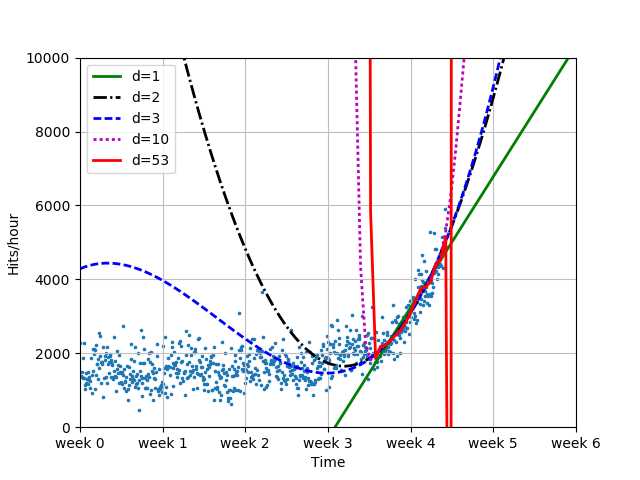
# 全模型转折点后拟合
fb1 = fb
fb2 = sp.poly1d(sp.polyfit(xb, yb, 2))
fb3 = sp.poly1d(sp.polyfit(xb, yb, 3))
fb10 = sp.poly1d(sp.polyfit(xb ,yb, 10))
fb100 = sp.poly1d(sp.polyfit(xb, yb, 100))
print("全模型转折点后误差统计:")
for f in [fb1, fb2, fb3, fb10, fb100]:
print("Error d=%i: %f" % (f.order, error(f, xb, yb)))
# 转折点后数据6周预测
plot_models(
x, y, [fb1, fb2, fb3, fb10, fb100], os.path.join("..", "1400_01_07.png"),
mx=sp.linspace(0, 6*7*24, 100),
ymax=10000, xmin=0)
sp.random.permutation()这个函数返回打乱的input
import scipy as sp
sp.random.permutation([1,2,3,4,5])
# Out[3]:
# array([4, 5, 1, 2, 3])
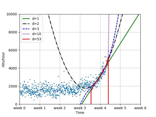
30%用于测试,70%用于拟合,这里随机分离数据
‘‘‘
转折点后数据
部分用于训练
部分用于测试
‘‘‘
frac = 0.3
split_idx = int(frac*len(xb))                             # 30%的数据量
shuffled = sp.random.permutation(list(range(len(xb))))    # 全xb的index乱序
test = sorted(shuffled[:split_idx])                       # 乱序index提取前30%,后排序
train = sorted(shuffled[split_idx:])                      # 乱序index提取后70%。后排序
拟合对比:
fbt1 = sp.poly1d(sp.polyfit(xb[train], yb[train], 1))
fbt2 = sp.poly1d(sp.polyfit(xb[train], yb[train], 2))
fbt3 = sp.poly1d(sp.polyfit(xb[train], yb[train], 3))
fbt10 = sp.poly1d(sp.polyfit(xb[train], yb[train], 10))
fbt100 = sp.poly1d(sp.polyfit(xb[train], yb[train], 100))

print("测试点误差:")
for f in [fbt1, fbt2, fbt3, fbt10, fbt100]:
    print("Error d=%i: %f" % (f.order, error(f, xb[test], yb[test])))
# 绘制部分训练模型拟合图
plot_models(x, y, [fbt1, fbt2, fbt3, fbt10, fbt100], os.path.join(‘..‘, ‘1400_01_08.png‘),
            mx=sp.linspace(0, 6*7*24),
            ymax=10000, xmin=0)
优化器解方程:
from scipy.optimize import fsolve
# 想要预测访问量100000的时间
print(fbt2)
print(fbt2-100000)
reached_max = fsolve(fbt2 - 100000, 800) / (7*24)
print("100,000 hits/hour excpeted at week %f" % reached_max)
『Python』MachineLearning机器学习入门_极小的机器学习应用
标签:数值 http plot 索引 脚本 互联网公司 com 对比 大小
原文地址:http://www.cnblogs.com/hellcat/p/6885215.html