标签:ant ica show 宽度 sed ict first 定义 increase
1. Introduction
A good edge detector must produce high quality edge maps, and it must run very fast. The speed of the detector is especially important for real-time computer vision and image processing applications. Among the existing edge detectors, Canny is generally considered to produce the best results, and is assumed to be the de-facto edge detector by the computer vision and image processing community. OpenCV implementation of Canny (cvCanny function) is the fastest known implementation of this famous edge detector, and is used by many real-time computer vision and image processing applications.
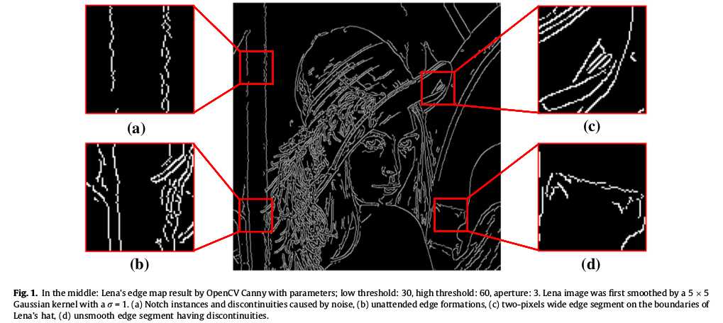
(a)噪声引起的切口实例和不连续性;(b)无人值守的边缘形态;(c)Lena’s帽子边界上的两个像素宽的边缘段;(d)未平滑的边缘段不连续的。
图1显示了著名的Lena图像的边缘图,该图像由opencv Canny获得,其中一些低质量的边缘片段已被放大显示。显然,边缘图本身是低质量的,由边缘线段组成,其中包括参差不齐的、不连续、无人值守的、多像素宽度的边缘。这是因为传统的边缘检测器,包括Canny算法,以孤立的和单独的方式评估像素,通常忽略像素间的关系,从而导致这种不连续性,单个和无人值守的边缘线段的构成。
对现有边缘检测实时性能的应用评价已经清楚地显示为一种新的边缘检测,需满足以下要求:(1)跑得很快,即实时性,(2)生产高质量的边缘图由相干的,连续的,本地化,1个像素宽的边缘。下面,我们提出边缘绘制(ED)[ 1 ]作为一种新的非正统的边缘或边界检测算法,满足这两个要求。ED不仅与传统的二值边缘图相区别,而且以矢量形式输出边缘图作为一组边缘段,每个边缘段由一个连续的像素链组成。
2. Edge Drawing algorithm (ED)
ED works on grayscale images and is comprised of four main steps:
(1) Suppression of noise by Gaussian filtering.
(2) Computation of the gradient magnitude and edge direction
maps.
(3) Extraction of the anchors.
(4) Connecting the anchors by smart routing.
2.1. Gaussian filtering
the very first step of ED is similar to most image processing methods: we convolve the image with a Gaussian kernel to suppress noise and smooth out the image. For all results given in this paper, a 5 × 5 Gaussian kernel with  = 1 is used.
2.2. Computation of the gradient magnitude and edge direction maps
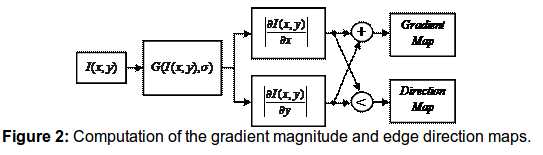
Figure 2 depicts the computation of the gradient magnitude and edge direction maps. Using the smoothed image, we compute the horizontal and vertical gradients, Gx and Gy, respectively. Any of the well-known gradient operators, e.g., Prewitt, Sobel, Scharr, etc., can be used at this step. The gradient magnitude G at a pixel is then obtained by simply adding Gx and Gy, i.e., G = |Gx| + |Gy|. Simultaneously with the gradient magnitude map, the edge direction map is also computed by simply comparing the horizontal and vertical gradients at each pixel. If the horizontal gradient is bigger, i.e., |Gx| >= |Gy|, a vertical edge is assumed to pass through the pixel. Otherwise, a horizontal edge is assumed to pass through the pixel. So, the gradient angle at a pixel is assumed to be either 0 or 90 degrees. Our experiments have shown that using two gradient angles were enough to smartly route the anchor linking process. Increasing the number of gradient angles simply increases the computational time without aiding the linking process.我们的实验表明,使用两个梯度角足以巧妙地锚定连接过程。增加梯度角的数目只是增加了计算时间而不帮助连接过程。
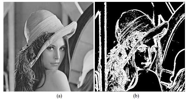
Figure 3: (a) Input image Lena, (b)Thresholded image with respect to gradient magnitudes. The Sobel operator and a threshold of 36 were used to obtain this image.
为了帮助我们忽略非边缘像素并加快计算速度,我们对梯度图进行阈值化,消除所谓的“弱”像素。这非常类似于Canny通过低阈值消除弱像素[ 3 ]:回想一下,在计算梯度图之后,Canny消除了梯度值小于用户定义的低阈值的像素。这些像素不包含边缘元素(边缘像素)。我们使用相同的想法,并消除那些像素的梯度幅度小于一个特定的用户定义的阈值。图3(a)显示了Lena图像,图3(b)显示相应的阈值梯度图。为了获得这个梯度图,我们使用Sobel算子和36的梯度阈值。黑色像素是Sobel算子产生小于36的梯度值的所有像素,所有其他像素都被标记为白色。我们称之为“边缘区域”图像。所有图像的边缘像素必须位于边缘区域的边界。消除的黑色像素不包含边缘像素。
2.3. Extraction of the anchors
高斯滤波和梯度图计算,ED前两个步骤与大多数边缘检测算法相似。边缘区域的图像而计算后,ED遵循一个非常非正统的方法:不是测试边缘区域内的单个像素成为边缘素,ED像素子集的第一个点(称为锚),然后将这些锚连接起来由一个启发式智能路算法( a heuristic smart routing algorithm)。直观地说,锚对应梯度图的峰(maximas)。如果你在3D中看到梯度图,锚就会成为山脉的顶点。
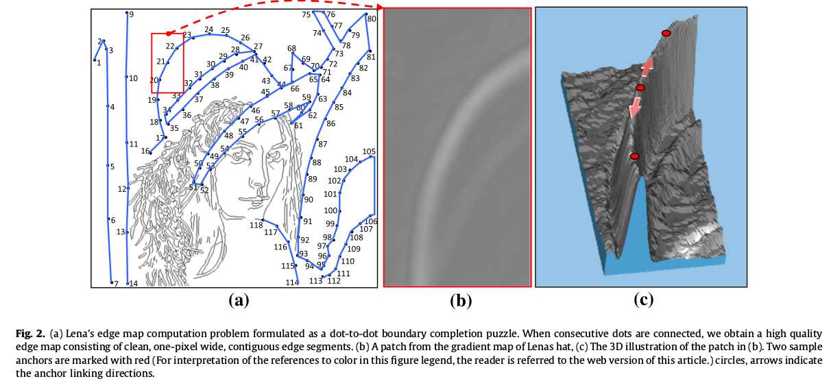
(a)Lena’s边缘图计算问题,它是一个点到点边界完成的拼图。当连续点连接时,我们得到一个高质量的边缘映射,由干净的、一个像素宽的、连续的边缘部分组成;(b)Lena’s帽子的梯度地图碎片;(c)碎片(b)在三维图。两个样品锚用红色圆圈标记,箭头表示锚点连接方向。
检测锚点的算法:
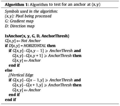
算法1显示了检查作为锚的像素(x,y)的算法。由于锚必须是梯度图的一个顶点,所以我们只需将像素的梯度值与它相邻的进行比较。对于水平边缘,比较上下邻居;对于垂直边缘,比较左和右邻居。如果像素的梯度值大于其相邻值通过一定的阈值(ANCHOR_THRESH),此像素标记为锚。通过改变锚阈值,可以调整锚的数量。此外,锚定测试可以在不同的扫描间隔,即每行/列,每两行/列等。增加锚的数量将增加边缘地图的细节,反之亦然。我们还注意到,锚提取是一个类属过程,其他的锚提取方法可以用来代替表1中给出的方法。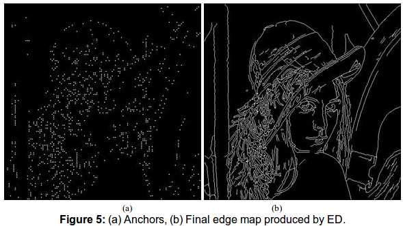
图5(a)显示了锚阈值为8的Lena图像的一组锚,以及扫描间隔为4;也就是说,每第四行或列已被扫描以测试锚。扫描每一行和列将产生更多的锚。增加扫描间隔将减少锚的数量。一般的经验法则如下:如果请求图像的所有细节,应该使用1的扫描间隔。如果只请求长的边缘(即对象边界的骨架),则可以使用较大的扫描间隔。因此,通过改变这个参数,可以很容易地调整最终边缘图中的细节量。
2.4. Connecting the anchors by smart routing
ED的最后一步也是最关键的一步是通过连接它们之间的锚来绘制边缘。由于在这一步中,通过使用算法前三个步骤中收集的信息构造了边缘图,因此这一步骤值得特别注意。
连接连续的锚,我们只是从一个高峰(锚)定到下一个走过梯度图的山脉。这个过程由算法的步骤2中计算的梯度幅度和边缘方向图来指导。
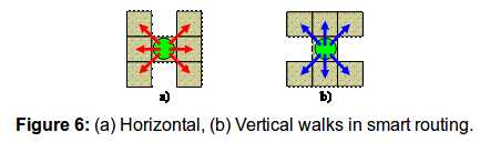
The smart routing process works as follows: 从锚点开始,我们查看通过锚的边缘的方向。如果水平边通过锚,我们开始连接过程,通过向左和右边行走(参见图6(a))。如果垂直边通过锚点,我们将开始上下移动链接过程(参见图6(b))。在移动过程中,只有3个紧邻的邻居被考虑,最大梯度值的一个被选中。移动在2个条件下停止:
(1)我们离开的边缘地区,即当前像素的阈值梯度值是0。
(2)我们遇到一个先前检测到的边缘像素。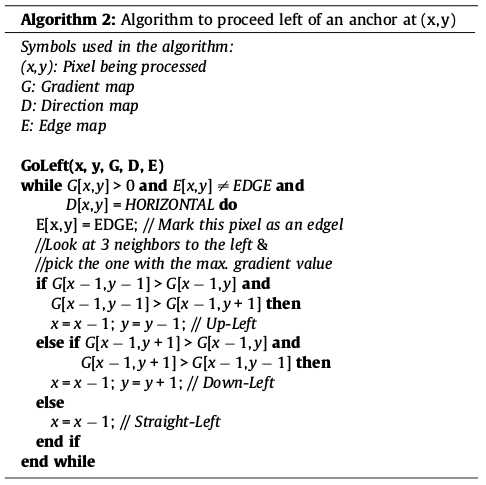
标签:ant ica show 宽度 sed ict first 定义 increase
原文地址:http://www.cnblogs.com/Jessica-jie/p/7679182.html