标签:operator target imp help more create rcp efault notebook
Welcome to your week 4 assignment (part 1 of 2)! You have previously trained a 2-layer Neural Network (with a single hidden layer). This week, you will build a
deep neural network, with as many layers as you want!
After this assignment you will be able to:
Notation:
Let‘s get started!
Let‘s first import all the packages that you will need during this assignment.
import numpy as np
import h5py
import matplotlib.pyplot as plt
from testCases_v3 import *
from dnn_utils_v2 import sigmoid, sigmoid_backward, relu, relu_backward

%matplotlib inline
plt.rcParams[‘figure.figsize‘] = (5.0, 4.0) # set default size of plots
plt.rcParams[‘image.interpolation‘] = ‘nearest‘
plt.rcParams[‘image.cmap‘] = ‘gray‘

%load_ext autoreload
%autoreload 2

np.random.seed(1)
To build your neural network, you will be implementing several "helper functions". These helper functions will be used in the next assignment to build a two-layer neural network and an L-layer neural network. Each small helper function you will implement will have detailed instructions that will walk you through the necessary steps. Here is an outline of this assignment, you will:
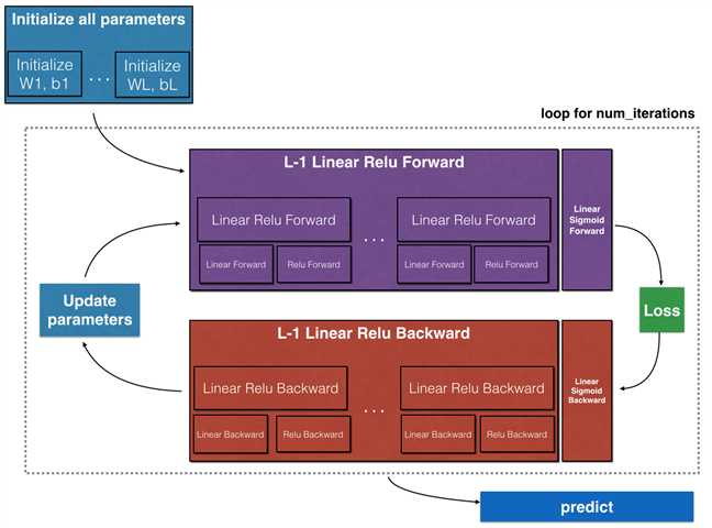
Note that for every forward function, there is a corresponding backward function. That is why at every step of your forward module you will be storing some values in a cache. The cached values are useful for computing gradients. In the backpropagation module you will then use the cache to calculate the gradients. This assignment will show you exactly how to carry out each of these steps.
You will write two helper functions that will initialize the parameters for your model. The first function will be used to initialize parameters for a two layer model. The second one will generalize this initialization process to LL layers.
Exercise: Create and initialize the parameters of the 2-layer neural network.
Instructions:
np.random.randn(shape)*0.01 with the correct shape.np.zeros(shape).
# GRADED FUNCTION: initialize_parameters

def initialize_parameters(n_x, n_h, n_y):
    """
    Argument:
    n_x -- size of the input layer
    n_h -- size of the hidden layer
    n_y -- size of the output layer

    Returns:
    parameters -- python dictionary containing your parameters:
                    W1 -- weight matrix of shape (n_h, n_x)
                    b1 -- bias vector of shape (n_h, 1)
                    W2 -- weight matrix of shape (n_y, n_h)
                    b2 -- bias vector of shape (n_y, 1)
    """

    np.random.seed(1)

    ### START CODE HERE ### (≈ 4 lines of code)
    W1 = np.random.randn(n_h,n_x)*0.01
    b1 = np.zeros((n_h,1))
    W2 = np.random.randn(n_y,n_h)*0.01
    b2 = np.zeros((n_y,1))
    ### END CODE HERE ###

    assert(W1.shape == (n_h, n_x))
    assert(b1.shape == (n_h, 1))
    assert(W2.shape == (n_y, n_h))
    assert(b2.shape == (n_y, 1))

    parameters = {"W1": W1,
                  "b1": b1,
                  "W2": W2,
                  "b2": b2}

    return parameters
parameters = initialize_parameters(3,2,1)
print("W1 = " + str(parameters["W1"]))
print("b1 = " + str(parameters["b1"]))
print("W2 = " + str(parameters["W2"]))
print("b2 = " + str(parameters["b2"]))
W1 = [[ 0.01624345 -0.00611756 -0.00528172]
 [-0.01072969  0.00865408 -0.02301539]]
b1 = [[ 0.]
 [ 0.]]
W2 = [[ 0.01744812 -0.00761207]]
b2 = [[ 0.]]
Expected output:
| W1 | [[ 0.01624345 -0.00611756 -0.00528172] [-0.01072969 0.00865408 -0.02301539]] |
| b1 | [[ 0.] [ 0.]] |
| W2 | [[ 0.01744812 -0.00761207]] |
| b2 | [[ 0.]] |
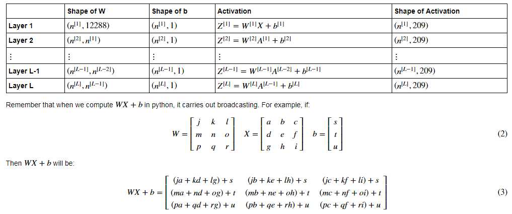
The initialization for a deeper L-layer neural network is more complicated because there are many more weight matrices and bias vectors. When completing the initialize_parameters_deep, you should make sure that your dimensions match between each layer. Recall that n[l]n[l] is the number of units in layer ll. Thus for example if the size of our input XX is (12288,209)(12288,209) (with m=209m=209 examples) then:
Exercise: Implement initialization for an L-layer Neural Network.
Instructions:
np.random.rand(shape) * 0.01.np.zeros(shape).layer_dims. For example, the layer_dims for the "Planar Data classification model" from last week would have been [2,4,1]: There were two inputs, one hidden layer with 4 hidden units, and an output layer with 1 output unit. Thus means W1‘s shape was (4,2), b1 was (4,1), W2 was (1,4) and b2 was (1,1). Now you will generalize this to LL layers! if L == 1:
parameters["W" + str(L)] = np.random.randn(layer_dims[1], layer_dims[0]) * 0.01
parameters["b" + str(L)] = np.zeros((layer_dims[1], 1))# GRADED FUNCTION: initialize_parameters_deep def initialize_parameters_deep(layer_dims): """ Arguments: layer_dims -- python array (list) containing the dimensions of each layer in our network Returns: parameters -- python dictionary containing your parameters "W1", "b1", ..., "WL", "bL": Wl -- weight matrix of shape (layer_dims[l], layer_dims[l-1]) bl -- bias vector of shape (layer_dims[l], 1) """ np.random.seed(3) parameters = {} L = len(layer_dims) # number of layers in the network for l in range(1, L): #my# range(1,3) [1,2] range(10) presents: range(0, 10) [0, 1, 2, 3, 4, 5, 6, 7, 8, 9] ### START CODE HERE ### (≈ 2 lines of code) parameters[‘W‘ + str(l)] = np.random.randn(layer_dims[l],layer_dims[l-1]) * 0.01 parameters[‘b‘ + str(l)] = np.zeros((layer_dims[l],1)) ### END CODE HERE ### assert(parameters[‘W‘ + str(l)].shape == (layer_dims[l], layer_dims[l-1])) assert(parameters[‘b‘ + str(l)].shape == (layer_dims[l], 1)) return parameters
parameters = initialize_parameters_deep([5,4,3])
print("W1 = " + str(parameters["W1"]))
print("b1 = " + str(parameters["b1"]))
print("W2 = " + str(parameters["W2"]))
print("b2 = " + str(parameters["b2"]))
Expected output:
| W1 | [[ 0.01788628 0.0043651 0.00096497 -0.01863493 -0.00277388] [-0.00354759 -0.00082741 -0.00627001 -0.00043818 -0.00477218] [-0.01313865 0.00884622 0.00881318 0.01709573 0.00050034] [-0.00404677 -0.0054536 -0.01546477 0.00982367 -0.01101068]] |
| b1 | [[ 0.] [ 0.] [ 0.] [ 0.]] |
| W2 | [[-0.01185047 -0.0020565 0.01486148 0.00236716] [-0.01023785 -0.00712993 0.00625245 -0.00160513] [-0.00768836 -0.00230031 0.00745056 0.01976111]] |
| b2 | [[ 0.] [ 0.] [ 0.]] |
Now that you have initialized your parameters, you will do the forward propagation module. You will start by implementing some basic functions that you will use later when implementing the model. You will complete three functions in this order:
The linear forward module (vectorized over all the examples) computes the following equations:
where A[0]=XA[0]=X.
Exercise: Build the linear part of forward propagation.
Reminder: The mathematical representation of this unit is Z[l]=W[l]A[l?1]+b[l]Z[l]=W[l]A[l?1]+b[l]. You may also find np.dot() useful. If your dimensions don‘t match, printing W.shape may help.
# GRADED FUNCTION: linear_forward

def linear_forward(A, W, b):
    """
    Implement the linear part of a layer‘s forward propagation.

    Arguments:
    A -- activations from previous layer (or input data): (size of previous layer, number of examples)
    W -- weights matrix: numpy array of shape (size of current layer, size of previous layer)
    b -- bias vector, numpy array of shape (size of the current layer, 1)

    Returns:
    Z -- the input of the activation function, also called pre-activation parameter
    cache -- a python dictionary containing "A", "W" and "b" ; stored for computing the backward pass efficiently
    """

    ### START CODE HERE ### (≈ 1 line of code)
    Z = np.dot(W,A) + b
    ### END CODE HERE ###

    assert(Z.shape == (W.shape[0], A.shape[1]))
    cache = (A, W, b)

    return Z, cache
A, W, b = linear_forward_test_case()

Z, linear_cache = linear_forward(A, W, b)
print("Z = " + str(Z))
Expected output:
| Z | [[ 3.26295337 -1.23429987]] |
Building your Deep Neural Network: Step by Step
标签:operator target imp help more create rcp efault notebook
原文地址:http://www.cnblogs.com/jiaxiangh/p/8000064.html