Finally pass all the Deeplearning.ai courses in March! I highly recommend it!
If you already know the basic then you may be interested in course 4 & 5, which shows many interesting cases in CNN and RNN. Altough I do think that 1 & 2 is better structured than others, which give me more insight into NN.
I have uploaded the assignment of all the deep learning courses to my GitHub. You can find the assignment for CNN here. Hopefully it can give you some help when you struggle with the grader. For a new course, you indeed need more patience to fight with the grader. Don‘t ask me how I know this ... >_<
I have finished the summary of the first course in my pervious post:
I will keep working on the others. Since I am using CNN at work recently, let‘s go through CNN first. Any feedback is absolutely welcomed! And please correct me if I make any mistake.
When talking about CNN, image application is usually what comes to our mind first. While actually CNN can be more generally applied to differnt data that fits certain assumption. what assumption? You will know later.
1. CNN Features
CNN stands out from traditional NN in 3 area:
- sparse interaction (connection)
- parameter sharing
- equivariant representation.
Actually the third feature is more like a result of the first 2 features. Let‘s go through them one by one.
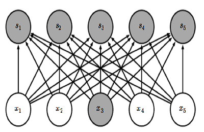
| Fully Connected NN | NN with Sparse connection |
|---|---|
 |
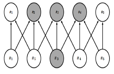 |
Sparse interaction, unlike fullly connected neural network, for Convolution layer each output is only connected to limited inputs like above. For a hidden layer that takes \(m\) neurons as input and \(n\) neurons as output, a fullly connected hidden layer has a weight matrix of size \(m*n\) to compute each ouput. When \(m\) is very big, the weigt can be a huge matrix. With sparse connection, only \(k\) input is connected to each output, leading to a decrease in computation scale from \(O(m*n)\) to \(O(k*n)\). And a decrease in memory usage from \(m*n\) to \(k*n\).
Parameter sharing has more insight when considered together with sparse connection. Becasue sparse connection creates segmentation among data. For example \(x_1\) \(x_5\) is independent in above plot due to sparse connection. However with parameter sharing, same weight matrix is used across all positions, leading to a hidden connectivity. Additionally, it can further reduces the memory storage of weight matrix from \(k*n\) to \(k\). Especially when dealing with image, from \(m*n\) to \(k\) can be a huge improvment in memory usage.
Equivariant representation is a result of parameter sharing. Because same weight matrix is used at different position across input. So the output is invaritate to parallel movemnt. Say \(g\) represent parallel shift and \(f\) is the convolution function, then \(f(g(x)) = g(f(x))\). This feature can be very useful when we only care about the presence of feature not their position. But on the other hand this can be a big flaw of CNN that it is not good at detecting position.
2. CNN Components
Given the above 3 features, let‘s talk about how to implement CNN.
(1).Kernel
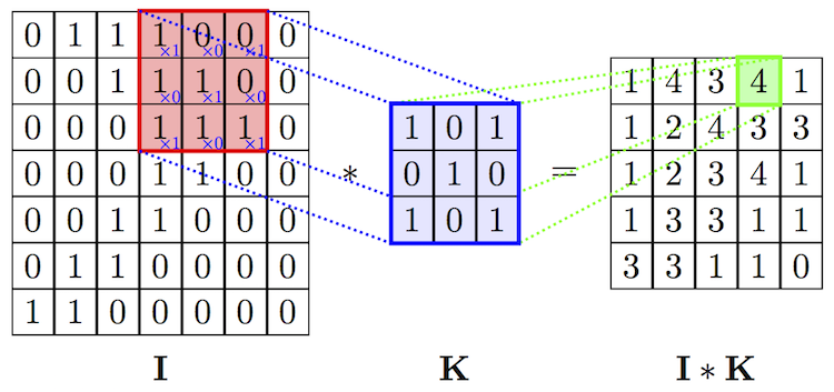
Kernel, or so-called filter, is the weight matrix in CNN. It implements element-wise computation across input matrix and output the sum. Kernel usually has a size that is much smaller than the original input so that we can take advantage of decrease in memory.
Below is a 2D input of convolution layer. It can be greyscale image, or multivarate timeseries.
When input is 3D dimension, we call the 3rd dimension Channel(volume). The most common case is the RGB image input, where each channel is a 2D matrix representing one color. See below:
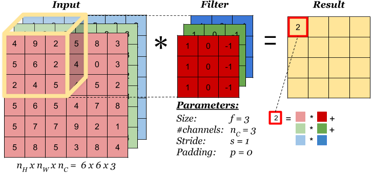
Please keep in mind that Kernel always have same number of channel as input! Therefore it leads to dimension reduction in all dimensions (unless you use 1*1 kernel). But we can have multiple kernels to capture differnt features. Like below, we have 2 kernels(filters), each has dimension (3,3,3).
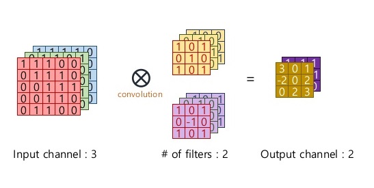
Dimension Cheatsheet of Kernel
- Input Dimension ( n_w, n_h, n_channel ). When n_channel = 1, it is a 2D input.
- Kernel Dimension ( n_k, n_k, n_channel ). Kernel is not always a square, it can be ( n_k1, n_k2, n_channel )
- Output Dimension (n_w - n_k + 1, n_h - n_k + 1, 1 )
- When we have n different kernels, output dimension will be (n_w - n_k + 1, n_h - n_k + 1, n)
(2). Stride
Like we mention before, one key advantage of CNN is to speeed up computation using dimension reduction. Can we be more aggresive on this ?! Yes we can use Stride! Basically stride is when moving kernel across input, it skips certain input by certain length.
We can easily tell how stride works by below comparison:
 No Stride
 Stride = 1
Thanks vdumoulin for such great animation. You can find more at his github
Stride can further speed up computation, but it will lose some feature in the output. We can consider it as output downsampling.
(3). Padding
Both Kernel and Stride function as dimension reduction technic. So for each convolution layer, the output dimension will always be smaller than input. However if we want to build a deep convolution network, we don‘t want the input size to shrink too fast. A small kernel can partly solve this problem. But in order to maintain certain dimension we need zero padding. Basically it is adding zero to your input, like below:
 Padding = 1
There is a few types of padding that are frequently used:
- Valid padding: no padding at all, output = input - (K - 1)
- Same padding: maintain samesize, output = input
- Full padding: each input is visited k times, output = input + (k - 1)
To summarize, We use \(s\) to denote stride, and \(p\) denotes padding. \(n\) is the input size, \(k\) is kernel size (kernel and input are both sqaure for simplicity). Then output dimension will be following:
\[\lfloor (n+2p-k)/s\rfloor +1\]
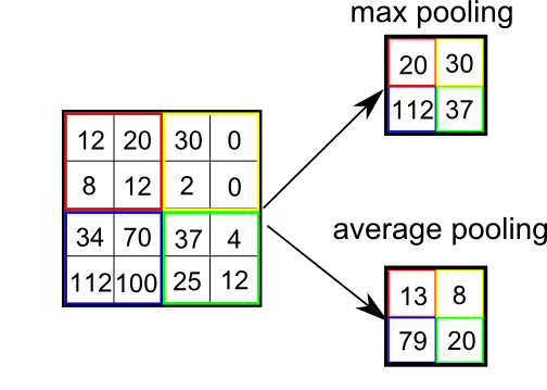
(4). Pooling
I remember in a latest paper of CNN, the author says that I can‘t explain why I add pooling layer, but a good CNN structure always comes with a pooling layer.
Pooling functions as a dimension reduction Technic. But unlike Kernel which reduces all dimensions, pooling keep channel dimension untouched. Therefore it can further accelerate computation.
Basicallly Pooling ouputs a certain statistics for a certain amoung of input. This introduces a feature stronger than Equivariant representation -- Invariant representation.
The mainly used Pooling is max and average pooling. And there is L2, and weighted average, and etc.
3. CNN structure
(1). Intuition of CNN
In Deep Learning book, author gives a very interesting insight. He consider convolution and pooling as a infinite strong prior distribution. The distribution indicates that all hidden units share the same weight, derived from certain amount of the input and have parallel invariant feature.
Under Bayesian statistics, prior distribuion is a subjective preference of the model based on experience. And the stronger the prior distribution is, the higher impact it will have on the optimal model. So before we use CNN, we have to make sure that our data fits the above assumption.
(2). classic structure
A classic convolution neural network has a convolutional layer, a non-linear activation layer, and a pooling layer. For deep NN, we can stack a few convolution layer together. like below
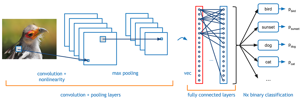
The above plot is taken from Adit Deshpande‘s A Beginner‘s Guide To Understanding Convolutional Neural Networks, one of my favoriate blogger of ML.
The interesting part of deep CNN is that deep hidden layer can receive more information from input than shallow layer, meaning although the direct connection is sparse, the deeper hidden neuron are still able to receive nearly all the features from input.
(3). To be continue
With learning more and more about NN, I gradually realize that NN is more flexible than I thought. It is like LEGO, convolution, pooling, they are just different basic tools with different assumption. You need to analyze your data and select tools that fits your assumption, and try combining them to improve performance interatively. Latrer I will open a new post to collect all the NN structure that I ever read about.
Reference
1 Vincent Dumoulin, Francesco Visin - A guide to convolution arithmetic for deep learning (BibTeX)
2 Adit Deshpande - A Beginner‘s Guide To Understanding Convolutional Neural Networks
3 Ian Goodfellow, Yoshua Bengio, Aaron Conrville - Deep Learning