标签:core def 回归 title att 实验 == dde bec
我们将实现一个简单的3层神经网络,我们不会仔细推到所需要的数学公式,但我们会给出我们这样做的直观解释。注意,此次代码并不能达到非常好的效果,可以自己进一步调整或者完成课后练习来进行改进。
# Package imports
import matplotlib.pyplot as plt
import numpy as np
import sklearn
import sklearn.datasets
import sklearn.linear_model
import matplotlib

# Display plots inline and change default figure size
%matplotlib inline
matplotlib.rcParams[‘figure.figsize‘] = (10.0, 8.0) # 指定matplotlib画布规模
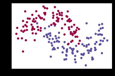
注意到,scikit-learn包包含了数据生成的代码,因此我们无需自己实现,直接采用其make_moons方法即可。下图中有两种类别的点,蓝点表示男患者,红点表示女患者,而xy坐标表示医学测量指标。我们的目的是去训练一个模型可以根据医学测量指标结果来划分男女患者,注意到图中的划分界限不是简单的线性的,因此采用简单的逻辑回归的效果合理不会很好。
# Generate a dataset and plot it
np.random.seed(0)
X, y = sklearn.datasets.make_moons(200, noise=0.20)
plt.scatter(X[:,0], X[:,1], s=40, c=y, cmap=plt.cm.Spectral)
为了证明上述观点我们来训练一个逻辑回归模型看看效果。输入是xy坐标,而输出是(0,1)二分类。我们直接使用scikit-learn包中的逻辑回归算法做预测。
# Train the logistic regression classifier
clf = sklearn.linear_model.LogisticRegressionCV()
clf.fit(X, y)
Out[3]:
LogisticRegressionCV(Cs=10, class_weight=None, cv=None, dual=False,
           fit_intercept=True, intercept_scaling=1.0, max_iter=100,
           multi_class=‘ovr‘, n_jobs=1, penalty=‘l2‘, random_state=None,
           refit=True, scoring=None, solver=‘lbfgs‘, tol=0.0001, verbose=0)
# Helper function to plot a decision boundary.
# If you don‘t fully understand this function don‘t worry, it just generates the contour plot below.
def plot_decision_boundary(pred_func):
    # Set min and max values and give it some padding
    x_min, x_max = X[:, 0].min() - .5, X[:, 0].max() + .5
    y_min, y_max = X[:, 1].min() - .5, X[:, 1].max() + .5
    h = 0.01
    # Generate a grid of points with distance h between them
    xx, yy = np.meshgrid(np.arange(x_min, x_max, h), np.arange(y_min, y_max, h))
    # Predict the function value for the whole gid
    Z = pred_func(np.c_[xx.ravel(), yy.ravel()])
    Z = Z.reshape(xx.shape)
    # Plot the contour and training examples
    plt.contourf(xx, yy, Z, cmap=plt.cm.Spectral)
    plt.scatter(X[:, 0], X[:, 1], c=y, cmap=plt.cm.Spectral)
# Plot the decision boundary
plot_decision_boundary(lambda x: clf.predict(x))
plt.title("Logistic Regression")
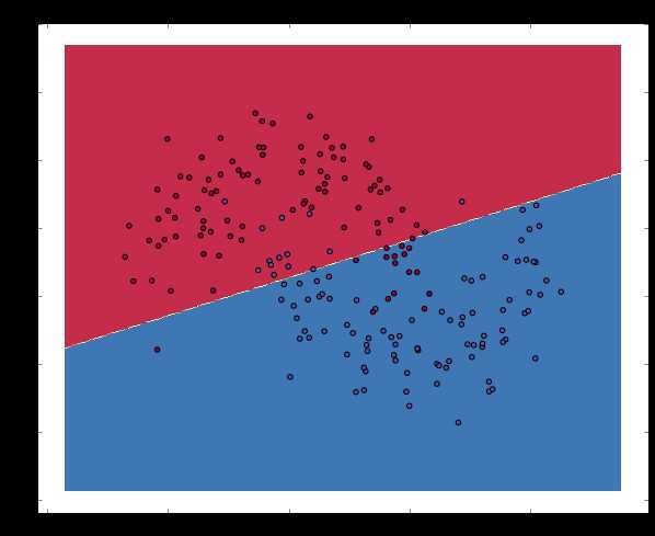
可以看到,逻辑回归使用一条直线尽可能好的分割这个二分类问题,但是由于原先数据本就不是线性可分的,因此效果并不好。
现在来构建一个有一个输入层一个隐藏层和一个输出层的简单三层神经网络来做预测。
神经网络通过下述公式进行预测。
$$
\begin{aligned}
z_1 & = xW_1 + b_1 \\
a_1 & = \tanh(z_1) \\
z_2 & = a_1W_2 + b_2 \\
a_2 & = \hat{y} = \mathrm{softmax}(z_2)
\end{aligned}
$$
学习参数是让我们的网络找到一组参数 ($W_1, b_1, W_2, b_2$)使得训练集上的损失最小化。现在我们来定义损失函数,这里我们使用常用的交叉熵损失函数,如下:
$$
\begin{aligned}
L(y,\hat{y}) = - \frac{1}{N} \sum_{n \in N} \sum_{i \in C} y_{n,i} \log\hat{y}_{n,i}
\end{aligned}
$$
而后我们使用梯度下降来最小化损失函数。我们将实现最简单的梯度下降算法,其实就是有着固定学习率的批量梯度下降。在实践中,梯度下降的一些变种如SGD(随机梯度下降)或者最小批次梯度下降往往有更好的表现。因此后续我们可以通过这些点来改进效果。
梯度下降需要计算出损失函数相对于我们要更新参数的梯度 $\frac{\partial{L}}{\partial{W_1}}$, $\frac{\partial{L}}{\partial{b_1}}$, $\frac{\partial{L}}{\partial{W_2}}$, $\frac{\partial{L}}{\partial{b_2}}$。为了计算这些梯度我们使用著名的反向传播算法,这种方法能够从输出开始有效地计算梯度。此处不细讲反向传播是如何工作的,只给出方向传播需要的公式,如下:
$$
\begin{aligned}
& \delta_3 = \hat{y} - y \\
& \delta_2 = (1 - \tanh^2z_1) \circ \delta_3W_2^T \\
& \frac{\partial{L}}{\partial{W_2}} = a_1^T \delta_3 \\
& \frac{\partial{L}}{\partial{b_2}} = \delta_3\\
& \frac{\partial{L}}{\partial{W_1}} = x^T \delta_2\\
& \frac{\partial{L}}{\partial{b_1}} = \delta_2 \\
\end{aligned}
$$
开始实现!
变量定义。
num_examples = len(X) # 训练集大小
nn_input_dim = 2 # 输入层维度
nn_output_dim = 2 # 输出层维度

# Gradient descent parameters (I picked these by hand)
epsilon = 0.01 # 梯度下降学习率
reg_lambda = 0.01 # 正规化权重
损失函数定义。
# Helper function to evaluate the total loss on the dataset
def calculate_loss(model):
    W1, b1, W2, b2 = model[‘W1‘], model[‘b1‘], model[‘W2‘], model[‘b2‘]
    # 前向传播,计算出预测值
    z1 = X.dot(W1) + b1
    a1 = np.tanh(z1)
    z2 = a1.dot(W2) + b2
    exp_scores = np.exp(z2)
    probs = exp_scores / np.sum(exp_scores, axis=1, keepdims=True)
    # 计算损失
    corect_logprobs = -np.log(probs[range(num_examples), y])
    data_loss = np.sum(corect_logprobs)
    # 损失值加入正规化
    data_loss += reg_lambda/2 * (np.sum(np.square(W1)) + np.sum(np.square(W2)))
    return 1./num_examples * data_loss
我们也实现了一个有用的用来计算网络输出的方法,其做了前向传播计算并且返回最高概率类别。
# Helper function to predict an output (0 or 1)
def predict(model, x):
    W1, b1, W2, b2 = model[‘W1‘], model[‘b1‘], model[‘W2‘], model[‘b2‘]
    # Forward propagation
    z1 = x.dot(W1) + b1
    a1 = np.tanh(z1)
    z2 = a1.dot(W2) + b2
    exp_scores = np.exp(z2)
    probs = exp_scores / np.sum(exp_scores, axis=1, keepdims=True)
    return np.argmax(probs, axis=1)
最后,使用批量梯度下降算法来训练我们的神经网络。
# This function learns parameters for the neural network and returns the model.
# - nn_hdim: Number of nodes in the hidden layer
# - num_passes: Number of passes through the training data for gradient descent
# - print_loss: If True, print the loss every 1000 iterations
def build_model(nn_hdim, num_passes=20000, print_loss=False):

    # 随机初始化权重
    np.random.seed(0)
    W1 = np.random.randn(nn_input_dim, nn_hdim) / np.sqrt(nn_input_dim)
    b1 = np.zeros((1, nn_hdim))
    W2 = np.random.randn(nn_hdim, nn_output_dim) / np.sqrt(nn_hdim)
    b2 = np.zeros((1, nn_output_dim))

    # 返回字典初始化
    model = {}

    # 对于每一个批次进行梯度下降
    for i in range(0, num_passes):

        # 前向传播
        z1 = X.dot(W1) + b1
        a1 = np.tanh(z1)
        z2 = a1.dot(W2) + b2
        exp_scores = np.exp(z2)
        probs = exp_scores / np.sum(exp_scores, axis=1, keepdims=True)

        # 反向传播
        delta3 = probs
        delta3[range(num_examples), y] -= 1
        dW2 = (a1.T).dot(delta3)
        db2 = np.sum(delta3, axis=0, keepdims=True)
        delta2 = delta3.dot(W2.T) * (1 - np.power(a1, 2))
        dW1 = np.dot(X.T, delta2)
        db1 = np.sum(delta2, axis=0)

        # 加入正则化
        dW2 += reg_lambda * W2
        dW1 += reg_lambda * W1

        # 梯度下降参数更新
        W1 += -epsilon * dW1
        b1 += -epsilon * db1
        W2 += -epsilon * dW2
        b2 += -epsilon * db2

        # 分配新权重
        model = { ‘W1‘: W1, ‘b1‘: b1, ‘W2‘: W2, ‘b2‘: b2}

        # Optionally print the loss.
        # This is expensive because it uses the whole dataset, so we don‘t want to do it too often.
        if print_loss and i % 1000 == 0:
          print("Loss after iteration %i: %f" %(i, calculate_loss(model)))

    return model
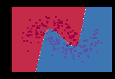
# Build a model with a 3-dimensional hidden layer
model = build_model(3, print_loss=True)

# Plot the decision boundary
plot_decision_boundary(lambda x: predict(model, x))
plt.title("Decision Boundary for hidden layer size 3")
Loss after iteration 0: 0.432387
Loss after iteration 1000: 0.068947
Loss after iteration 2000: 0.068926
Loss after iteration 3000: 0.071218
Loss after iteration 4000: 0.071253
Loss after iteration 5000: 0.071278
Loss after iteration 6000: 0.071293
Loss after iteration 7000: 0.071303
Loss after iteration 8000: 0.071308
Loss after iteration 9000: 0.071312
Loss after iteration 10000: 0.071314
Loss after iteration 11000: 0.071315
Loss after iteration 12000: 0.071315
Loss after iteration 13000: 0.071316
Loss after iteration 14000: 0.071316
Loss after iteration 15000: 0.071316
Loss after iteration 16000: 0.071316
Loss after iteration 17000: 0.071316
Loss after iteration 18000: 0.071316
Loss after iteration 19000: 0.071316
这看起来比逻辑回归的效果好多了!
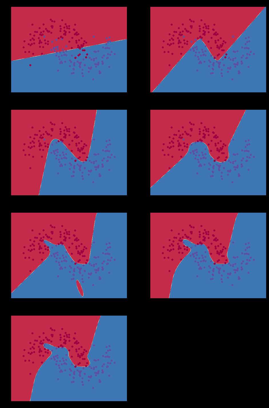
plt.figure(figsize=(16, 32))
hidden_layer_dimensions = [1, 2, 3, 4, 5, 20, 50]
for i, nn_hdim in enumerate(hidden_layer_dimensions):
    plt.subplot(5, 2, i+1)
    plt.title(‘Hidden Layer size %d‘ % nn_hdim)
    model = build_model(nn_hdim)
    plot_decision_boundary(lambda x: predict(model, x))
plt.show()
我们给出了一些练习。
使用模拟退火算法更新学习率,公式为$epsilon=\frac{epsilon_0}{1+d \times t}$。
# This function learns parameters for the neural network and returns the model.
# - nn_hdim: Number of nodes in the hidden layer
# - num_passes: Number of passes through the training data for gradient descent
# - print_loss: If True, print the loss every 1000 iterations
# - d: the decay number of annealing schedule
def build_model(nn_hdim, num_passes=20000, print_loss=False, d=10e-3):

    # Initialize the parameters to random values. We need to learn these.
    np.random.seed(0)
    W1 = np.random.randn(nn_input_dim, nn_hdim) / np.sqrt(nn_input_dim)
    b1 = np.zeros((1, nn_hdim))
    W2 = np.random.randn(nn_hdim, nn_output_dim) / np.sqrt(nn_hdim)
    b2 = np.zeros((1, nn_output_dim))

    # This is what we return at the end
    model = {}

    # Gradient descent. For each batch...
    for i in range(0, num_passes):

        # Forward propagation
        z1 = X.dot(W1) + b1
        a1 = np.tanh(z1)
        z2 = a1.dot(W2) + b2
        exp_scores = np.exp(z2)
        probs = exp_scores / np.sum(exp_scores, axis=1, keepdims=True)

        # Backpropagation
        delta3 = probs
        delta3[range(num_examples), y] -= 1
        dW2 = (a1.T).dot(delta3)
        db2 = np.sum(delta3, axis=0, keepdims=True)
        delta2 = delta3.dot(W2.T) * (1 - np.power(a1, 2))
        dW1 = np.dot(X.T, delta2)
        db1 = np.sum(delta2, axis=0)

        # Add regularization terms (b1 and b2 don‘t have regularization terms)
        dW2 += reg_lambda * W2
        dW1 += reg_lambda * W1

        epsilon_ = epsilon / (1+d*i)
        # Gradient descent parameter update
        W1 += -epsilon_ * dW1
        b1 += -epsilon_ * db1
        W2 += -epsilon_ * dW2
        b2 += -epsilon_ * db2

        # Assign new parameters to the model
        model = { ‘W1‘: W1, ‘b1‘: b1, ‘W2‘: W2, ‘b2‘: b2}

        # Optionally print the loss.
        # This is expensive because it uses the whole dataset, so we don‘t want to do it too often.
        if print_loss and i % 1000 == 0:
          print("Loss after iteration %i: %f" %(i, calculate_loss(model)))

    return model
Loss after iteration 0: 0.432387
Loss after iteration 1000: 0.081007
Loss after iteration 2000: 0.075384
Loss after iteration 3000: 0.073729
Loss after iteration 4000: 0.072895
Loss after iteration 5000: 0.072376
Loss after iteration 6000: 0.072013
Loss after iteration 7000: 0.071742
Loss after iteration 8000: 0.071530
Loss after iteration 9000: 0.071357
Loss after iteration 10000: 0.071214
Loss after iteration 11000: 0.071092
Loss after iteration 12000: 0.070986
Loss after iteration 13000: 0.070894
Loss after iteration 14000: 0.070812
Loss after iteration 15000: 0.070739
Loss after iteration 16000: 0.070673
Loss after iteration 17000: 0.070613
Loss after iteration 18000: 0.070559
Loss after iteration 19000: 0.070509
http://www.wildml.com/2015/09/implementing-a-neural-network-from-scratch/
https://github.com/dennybritz/nn-from-scratch
计算机视觉学习记录 - Implementing a Neural Network from Scratch - An Introduction
标签:core def 回归 title att 实验 == dde bec
原文地址:https://www.cnblogs.com/CZiFan/p/9848940.html