标签:inner question guide gpu nal rate tricks ant problems
This is the first course of the deep learning specialization at Coursera which is moderated by moderated by DeepLearning.ai. The course is taught by Andrew Ng.
Introduction to deep learning
Be able to explain the major trends driving the rise of deep learning, and understand where and how it is applied today.
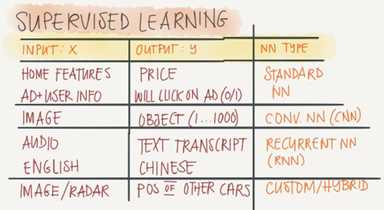
What is a (Neural Network) NN?
Single neuron == linear regression
Simple NN graph:
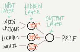
RELU stands for rectified linear unit is the most popular activation function right now that make deep NNs train faster now.
Hidden layers predicts connection between inputs automatically, that what deep learning is goog at.
Deep NN consists of more hidden layers (Deeper layers)
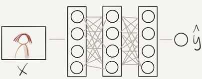
Each input will be connected to the hidden layer and the NN will decide the connections.
Supervised learning means we have the (X,Y) and we need to get the function that maps X to Y.
Supervised learning with neural networks
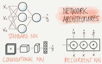
Different types of neural networks for supervised learning which includes:
CNN or convolutional neural networks (Useful in computer vision)
RNN or Recurrent neural networks (Useful in Speech recognition or NLP)
Standard NN (Useful for Structured data)
Hybrid/custom NN or a Collection of NNs types.
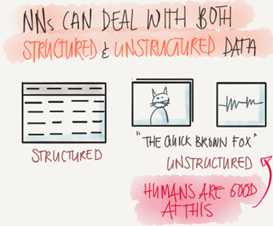
Structured data is like the databases and tables.
Unstructured data is like images, video, audio, and text.
Structured data gives more money because companies relies on prediction on its big data.
Why is deep learning taking off?
Deep learning is taking off for 3 reasons:
Using this image we can conclude:
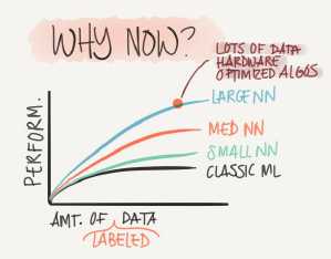
For small data NN can perform as Linear regression or SVM (Support vector machine)
For big data a small NN is better than SVM
For big data a big NN is better than a medium NN is better than small NN
Hopefully we have a lot of data because the world is using the computer a little bit more (Mobiles IOT(Internet of things))
GPUs
Powerful CPUS
Distributed computing
ASICs
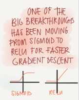
Creative algorithms has appeared that changed the way NN works.
(For example using RELU function is so much better than using SIGMOID function in training a NN because it helps with the vanishing gradient problem)
Neural Networks Basics
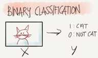
Learning to set up a machine learning problem with a neural networks mindset. Learn to use vectorization to speed up your models.
Binary classification

Here are some notations:
M is the number of training vectors
Nx is the size of input vector
Ny is the size of the out vector
X(1) is the first input vector
Y(1) is the first output vector
X=[x(1) x(2) … x(M)]
Y=[y(1) y(2) … y(M)]
We will use python in this course
In Numpy we can make matrices and make operations on them in a fast and reliable time
Logistic regression
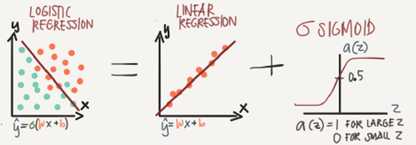
Algorithm is used for classification algorithm of 2 classses.
Equations:
Simple equation: y=w*x+b
If x is vector: y=w‘*x+b
If we need y to be in between 0 and 1 (probability): y=sigmoid(w‘x+b)
In some notations this might be used: y=sigmoid(w‘x)
While b is w0 of w and we add x0=1. But we won‘t use this notation in the course
In binary classification Y has to be between 0 and 1
In the last equation w is a vector of Nx and b is a real number
Logistic regression cost function
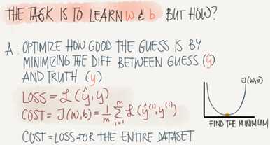
First loss function would be the square root error: L(y‘,y)=1/2(y‘-y)^2
But we won‘t use this notation because it leads us to optimization problem which is non convex, means it contains local optimum points.
This is the function that we will use: L(y‘,y)=-(y*log(y‘)+(1-y)*log(1-y‘))
To explain the last function lets see:
If y=1 è L(y‘,1)=-log(y‘)èwe want y‘ to be the largestèy‘ biggest value is 1
If y=0 è L(y‘,0)= -log(1-y‘)èwe want 1-y‘ to be the largestèy‘ to be smaller as possible because it can only has 1 value.
Then the Cost function will be: J(w,b)=(1/m)*sum(L(y‘[i],y[i]))
The loss function computes the error for single traing example; the cost function is the average of the loss function of the entire traing set.
Gradient Descent
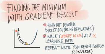
We want to predict w and b that minimize the cost function
Our cost function is convex
First we initialize w and b to 0,0 or initialize them to a random value in the convex function and then try to improve the values the reach minimum value.
In Logistic regression people always use 0,0 instead of random.
The gradient decent algorithm repeats: w=w-alpha*dw where alpha is the learning rate and dw is the derivative of w (change to w) The derivative is also the slope of w
Looks like greedy algorithms, the derivative give us the direction to improve our parameters
The actual equations we will implement:
w=w-alpha*d(J(w,b)/dw) (how much the function slopes in the w direction)
b=b-alpha*d(J(w,b)/db) (how much the function slopes in the d direction)
Derivatives
We will talk aboud some of required calculus.
You don‘t need to be a caculus geek to master deep learning but you‘ll need some skill from it.
Derivative of a linear line is its slope
Ex. f(a)=3a d(f(a))/d(a)=3
If a=2 then f(a)=6
If we move a little bit 1=2.001 then f(a)=6.003 means that we multiplied the derivative(Slope) to the movearea and added it to the last result.
More Derivatives examples
f(a)=a^2èd(f(a))/d(a)=2a
a=2èf(a)=4
a=2.0001èf(a)=4.0004 approx
f(a)=a^3èd(f(a))/d(a)=3a^2
f(a)=log(a)èd(f(a))/d(a)=1/a
To conclude, Derivative is the slope and slope is different in different points in the function thats why the derivative is a function
Computation graph
It‘s a graph that organizes the computation from left to righ
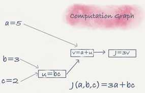 t
t
Derivatives with a Computation Graph
Calculus chain rule says: if x->y->z (x effect y and y effect z) Then d(z)/d(x) = d(z)/d(y) * d(y)/d(x)
The video illustrates a big example.
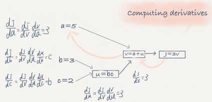
We compute the derivatives on a graph from right to left and it will be a lot more easier
dvar means the dervatives of a final output variable with respect to various intermediate quantities
Logistic Regression Gradient Descent
In the video he discussed the derivatives of gradient decent example for one sample with two features x1 and x2.
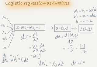
Gradient Descent on m Examples
Lets say we have these variables:
x1 Feature
x2 Feature
w1 weight of the first feature
w2 weight of the second feature
B Logistic Regression parameter
M Number of training exmaple
Y(i) Expected output of i
So we have:
z(i)=w1*x1+x2*w2+Bèa(i)=Sigmoid(z(i))èL(a(i),Y(i)))è-(Y(i)*log(a(i))+(1-Y(i))*log(1-a(i)))
Then from right to left we will calculate derivations compared to the result:
d(a)=d(l)/d(a)=-(y/a)+((1-y)/(1-a))
d(z)=d(l)/d(z)=a-y
d(w1)=x1*d(z)
d(w2)=x2*d(z)
d(B)=d(z)
From the above we can conclude the logistic regression pseudo code:
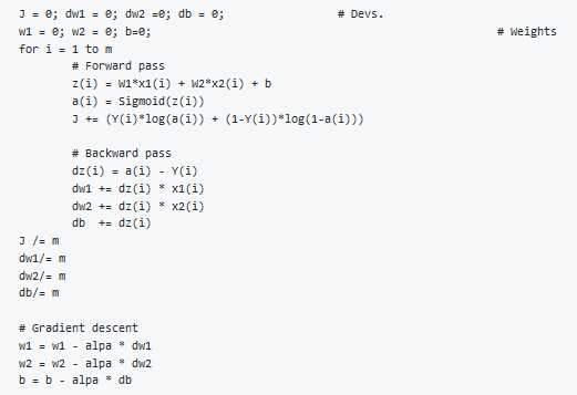
The above code should run for some iterations to minimize error
So there will be two inner loops to implement the logistic regression
Vectorization is so important deep learning to reduce loops. In the last code we can make the whole loop in one step using vectorization!
Vectorization
Deep learning shines when the dataset are big. However for loops will make you wait a lot for a result. That why we neede vectorization to get rid of some of our for loops.
Numpy library(dot) function is using vectorization by default.
The vectorization can be done on CPU or GPU thought the SIMD operation. But its faster on GPU.
Whenever possible avoid for loops.
Most of the Numpy library methods are vectorized version.
Vectorizing Logistic Regression
We will implement Logistic Regression using one for l oop then without any for loop.
As an input we have a matrix x and its [Nx,m] and a matrix Y and its [Ny,m]
We will then compute at instance [z1,z2,…zm]=w‘x+{b,b…b}. This can be written in python as
z=np.dot(w.T,x)+b #vectorization Then broadcasting, Z shape is (1,m)
A=1/1+np.exp(-z) #vectorization, A shape is (1,m)
Vectorizing Logistic Regression‘s Gradient Output:
dz=A-Y #vectorization,dz shape is (1,m)
dw=np.dot(X,dz.T)/m #vectorization, dw shape is (Nx,1)
db=dz.sum()/m #vectorization,dz shape is (1,1)
Notes on python and Numpy
In Numpy, obj.sum(axis=0) sums the columns while obj.sum(axis=1) sums the rows.
In Numpy, obj.reshape(1,4) changes the shape of the matrix by broadcasting the values.
Reshape is cheap in calculations so put it everywhere you‘re not sure about the calculations.
Broadcasting works when you do a matrix operation with matrices that does‘t match for the operation, in this case Numpy automatically makes the shapes ready for the operation by broadcasting the values.
Some tricks to eliminate all stange bugs in the code:
If you didn‘t specify the shape of a vector, it will take a shape of(m,) and the transpose operation won‘t work. You have to reshape it to (m,1)
Try to not use the rank one matrix in ANN
Don‘t hesitate to use assert(a.shape==(5,1)) to check if your matrix shape is the required one.
If you‘ve found a rank one matrix try to run reshape on it.
Jupyter/Ipython notebooks are so useful llibrary in python that makes it easy to integrate code and document at the same time. It runs in the browser and doesn‘t need an IDE to run.
To Compute the derivative of Sigmoid:

To make an image of (width,height,depth) be a vector, use this:

Gradient descent converges faster after normalization of the input matrices.
General Notes
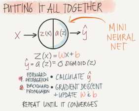
The mian steps for building a Neural Networks are:
Define the model structure (such as umber of input features and outputs)
Initialize the model‘s parameters
Loop
Calculate current loss (forward propagation)
Calculate current gradient (backward propagation)
Update parameters (gradient descent)
Shallow neural networks
Learn to build a neural network with one hidden layer, using forward propagation and backpropagation
Neural Networks Overivew
In logistic regeression we had:

In neural networks with one layer we will have:

x is the input vector (x1,x2,x3), and Y is the output variable (1*1)
NN is stack of logistic regression objects
Neural Network Representation
We will define the neural networks that has one hidden layer.
NN contains of input layers, hidden layers, out layers
Hidden layer means we cant see that layers in the trainging set
a0=x (the input layer)
a1 will represent the activation of the hidden neurons.
a2 will represent the output layer
we are talking about 2 layers NN. The input layer isn‘t counted.
Computing a Neural Network‘s Output
Equations of Hidden layers:
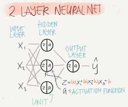
Here are some informations about the last image:
noOfHiddenNeurons=4
Nx=3
Shapes of the variables:
w1 is the matrix of the first hidden layer, it has a shape of (noOfHiddenNeurons,nx)
b1 is the matrix of the first hidden layer, it has a shape of (noOfHiddenNeurons,1)
z1 is the result of equation z1=x1*x+b, it has a shape of (noOfHiddenNeurons,1)
a1 is the reuslt of the equation a1=sigmoid(z1), it has a shape of (noOfHiddenNeurons,1)
w2 is the matrix of the second hidden layer, it has a shape of (1,noOfHiddenLayers)
b2 is the matrix of the second hidden layer, it has a shape of (1,1)
z2 is the result of the equation z2=w2*a1+b, it has a shape of (1,1)
a2 is the reuslt of the equation a2=sigmoid(z2), it has a shape of (1,1)
Vectorizing across multiple example
Pseudo code for forward propagation for 2 layers NN:

Lets say we have x on shape (Nx,m), So the new pseudo code

If you notice always m is the number of columns
In the last example we can call x,A0 for instance:

Activation functions
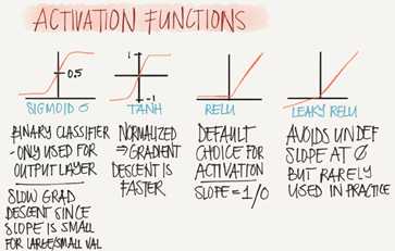
So far we are using sigmoid, but in some cases other functions can be a lot better.
Sigmoid can lead us to gradient decent problem where the updates are so low
Sigmoid activation function range is [0,1] A=1/(1+np.exp(-z)) #where z is the input matrix
Tanh activation function range is [-1,1] (shifted version of sigmoid function)
In Numpy we can implement Tanh using one of these methods: A=(np.exp(z)-np.exp(-z))/(np.exp(z)+np.exp(-z)) #where z is the input matrix
Or A=np.tanh(z) #where z is the input matrix
It turn out that using the Tanh function in hidden layers is far more better.(Because of the zero mean of the function)
Sigmoid or Tanh function disadvantage is that if the input is too small or too high, the slope will be near zero which will cause us the gradient decent problem.
One of the popular activation function that solved the slow gradient decent is the RELU function. RELU=max(0,z) #so if z is negative the slope is 0 and if z is positive the slope remians linear.
So here is some basic rule for choosing cactivation functoins, if your classification is between 0 and 1, use the output activation as sigmoid and others RELU
Leaky RELU activation function different of RELU is that if the input is negative the slope will be so small. It works as RELU but most people user RELU. Leak_RELU=max(0.01z,z) #the 0.01 can be a parameter for your algorithm.
In NN you will decide a lot of choices like:
No of hidden layers
No of neurons in each hidden layer.
Learing rate. (The most important parameter)
Activation function
And others..
It turns out there are no guide lines for that, You should try all activation function for example.
Why do you need no-linear activation functions?
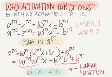
If we removed the activation function from our algorithm that can be called linear activation function.
Linear activation function will output linear activations
whatever hidden layers you add, the activation will be always linear like logistic regression(So its useless in a lot of complex problems)
You might use this in one place, If the output is real numbers, you can use linear activation function in the output layer.
Derivatives of activation functions
Derivation of Sigmoid activation function:

Derivation of Tanh activation function:

Derivation of RELU activation function:

Derivation of leaky RELU activation function:

Gradient descent for Neural Networks
In this section we will have the full back propagation of the neural network (Just the equations with no explanations)
Gradient descent algorithm:
NN parameters:
n[0]=Nx
n[1]=NoOfHiddenNeurons
n[2]=NoOfOutputNeurons=1
w1 shape is (n[1],n[0])
b1 shape is (n[1],1)
w2 shape is (n[2],n[1])
b2 shape is (n[2],1)
Cost function cost=cost(w1,b1,w2,b1)=(1/m)*sum(L(Y,A2))
Then Gradient descent:
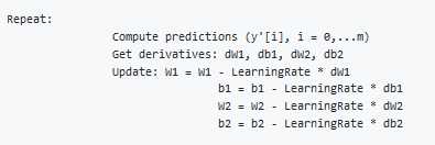
Forward propagation:

Back propagation(The new thing/derivations):

Random Initialization
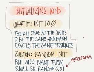
In logistic regression it wasn‘t important to initialize the weights randomly, while in NN we have to initialize them randomly.
If we initialize the weights with zeros in NNit won‘t work lets see why.
If we initialize w with zero, Then A1[:,1] will equal to A[:2], So Z[:,2] (We are talking in the middle layer)
Then all the hidden units will always updates the same.
To solve this we initialize the W‘s with a small random numbers:

We need small values because in sigmoid for example, if the number is big it will be 0 or 1 we will have flat parts. So learning will be so slow.
0.01 is alright for 1 hidden neurons, but if the NN is deep this number can be changed but will always be a small number.
Deep Neural Networks
understand the key computations underlying deep learning, use them to build and train deep neural networks, and apply it to computer vision.
Deep L-layer neural network
Shallow NN is a NN with one or two layers
Deep NN is a NN with three or more layers.
We will use the notation L to denote the number of layers in a NN
n[1] is the number of neurons in a specific layer 1
n[0] denotes the number of neurons input layer. n[L] denotes the number of neurons in output layer.
g[1] is the activation function
a[1]=g[1](z[l])
w[l] weights is used for z[l]
x=a[0], a[l]=y‘
These were the notation we will sue for deep neural network
So we have:
A vector n of shape (1,NoOfLayers+1)
A vector g of shape (1,NoOfLayers)
A list of different shapes w based on the number of neurons on the prevous and the current layer.
A list of different shapes b based on the number of neurons on the current layer.
Forward Propagation in a Deep Network
Forward propagation General rule for one input:

Forward propagation General rule for m inputs:

We can‘t compute the whole layers forward propagation without a for loop so its OK to have a for loop here.
The dimensions of the matrices are so important you need to figure it out.
Getting your matrix dimension right
The best way to debug your matrices dimension is by a pencil and paper.
Dimension of w is (n[l],n[l-1]). can be thought by Right to left
Dimension of b is (n[l],l)
dw has the same shape as w, while db is the same shape as b
Dimension of z[l],A[l],dz[l], and dA[l] is (n[l].m)
Why deep representations?
Why deep NN works well, we will discuss this question in this section
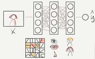
Deep NN makes relations with data from simpler to complex. In each layer it tries to make a relation between the previous layer
Face recognition application:
ImageàEdgesèFace partsèFacesèdesired face
Audio recognition application
AudioèLow level sound features like(sss,bb)èPhonemesèWordsèSentences
Neural Researchers thinks that deep neural networks thinks like brains (SimpleèComplex)
Circuit theory and deep learning
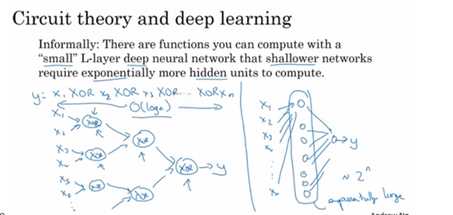
When starting on an application don‘t start directly by dozens of hidden layers. Try the simplest solutions(L Regression) then try the parameters then try the shallow neural network and so on.
Building blocks of deep neural networks
Forward and back propagation for a layer l:
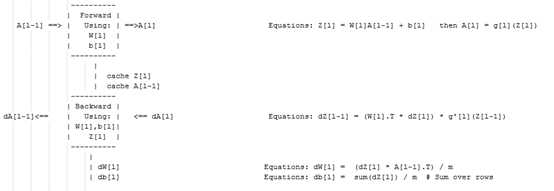
Deep NN blocks:
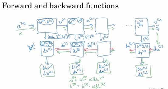
Forward and Backward Propagation
Pseudo code for forward propagation for layer I:

Pseudo code for back propagation for layer l:

If we have used our loss function then:

Parameters Vs Hyperparameters
Main parameters of NN is w and b
Hyper parameters (parameters that control the algorithm) are like:
Learning rate
Number of iteration.
Number of hidden layers L
Number of hidden units n
Choice of activation function
You have to try values yourself of hyper paramters
In the old days they thought that learning rate is a paramter while now all knows it‘s a hyper paramter
On the next course we will see how to optimize hyperparameters
What does this have to do with brain
No Human today understand how a human brain neuron works
No Human today know exactly how many neurons on the brain
NN is a small representation of how brain work. The most near model of human brain is in the computer vision (CNN)
Neural Networks and Deep Learning
标签:inner question guide gpu nal rate tricks ant problems
原文地址:https://www.cnblogs.com/kexinxin/p/9904526.html