Pytorch入门实战二：LeNet、AleNet、VGG、GoogLeNet、ResNet模型详解

时间：2019-03-06 00:32:20 阅读：616 评论：0 收藏：0 [点我收藏+]

LeNet

　　1998年，LeCun提出了第一个真正的卷积神经网络，也是整个神经网络的开山之作，称为LeNet，现在主要指的是LeNet5或LeNet-5，如图1.1所示。它的主要特征是将卷积层和下采样层相结合作为网络的基本机构，如果不计输入层，该模型共7层，包括2个卷积层，2个下采样层，3个全连接层。

技术图片

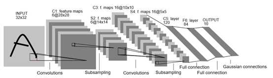
图1.1

　　注：由于在接入全连接层时，要将池化层的输出转换成全连接层需要的维度，因此，必须清晰的知道全连接层前feature map的大小。卷积层与池化层输出的图像大小，其计算如图1.2所示。

技术图片

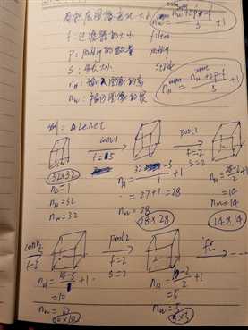
图1.2

　　本次利用pytorch实现整个LeNet模型，图中的Subsampling层即可看作如今的池化层，最后一层（输出层）也当作全连接层进行处理。

 1 import torch as torch
 2 import torch.nn as nn
 3 class LeNet(nn.Module):
 4     def __init__(self):
 5         super(LeNet,self).__init__()
 6         layer1 = nn.Sequential()
 7         layer1.add_module(‘conv1‘,nn.Conv2d(1,6,5))
 8         layer1.add_module(‘pool1‘,nn.MaxPool2d(2,2))
 9         self.layer1 = layer1
10 
11         layer2 = nn.Sequential()
12         layer2.add_module(‘conv2‘,nn.Conv2d(6,16,5))
13         layer2.add_module(‘pool2‘,nn.MaxPool2d(2,2))
14         self.layer2 = layer2
15 
16         layer3 = nn.Sequential()
17         layer3.add_module(‘fc1‘,nn.Linear(16*5*5,120))
18         layer3.add_module(‘fc2‘,nn.Linear(120,84))
19         layer3.add_module(‘fc3‘,nn.Linear(84,10))
20         self.layer3 = layer3
21 
22     def forward(self, x):
23         x = self.layer1(x)
24         x = self.layer2(x)
25         x = x.view(x.size(0),-1)#转换（降低）数据维度，进入全连接层
26         x = self.layer3(x)
27         return x
28 #代入数据检验
29 y = torch.randn(1,1,32,32)
30 model = LeNet()
31 model(y)

AlexNet

　　在2010年，斯坦福大学的李飞飞正式组织并启动了大规模视觉图像识别竞赛（ImageNet Large Scale Visual Recognition Challenge，ILSVRC）。在2012年，Alex Krizhevsky、Ilya Sutskever提出了一种非常重要的卷积神经网络模型，它就是AlexNet，如图1.3所　　示，在ImageNet竞赛上大放异彩，领先第二名10%的准确率夺得了冠军，吸引了学术界与工业界的广泛关注。

　　AlexNet神经网络相比LeNet：

1、使用ReLU激活函数。在AlexNet之前，神经网络一般都使用sigmoid或tanh作为激活函数，这类函数在自变量非常大或者非常小时，函数输出基本不变，称之为饱和函数。为了提高训练速度，AlexNet使用了修正线性函数ReLU，它是一种非饱和函数，与 sigmoid 和tanh 函数相比，ReLU分片的线性结构实现了非线性结构的表达能力，梯度消失现象相对较弱，有助于训练更深层的网络。
2、使用GPU训练。与CPU不同的是，GPU转为执行复杂的数学和几何计算而设计，AlexNet使用了2个GPU来提升速度，分别放置一半卷积核。
3、局部响应归一化。AlexNet使用局部响应归一化技巧，将ImageNet上的top-1与top-5错误率分别减少了1.4%和1.2%。
4、重叠池化层。与不重叠池化层相比，重叠池化层有助于缓解过拟合，使得AlexNet的top-1和top-5错误率分别降低了0.4%和0.3%。
5、减少过拟合。AlexNet使用了数据扩增与丢失输出两种技巧。数据扩增：a、图像的平移、翻转，b、基于PCA的RGB强度调整。丢失输出技巧（DropOut层），AlexNet以0.5的概率将两个全连接层神经元的输出设置为0，有效阻止了过拟合现象的发生。

技术图片

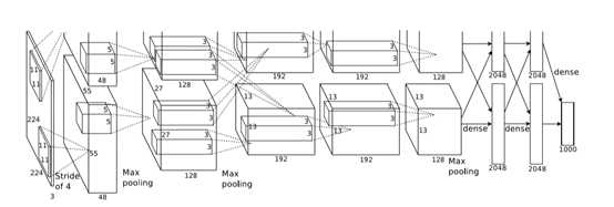
图1.3

　　利用pytorch实现AlexNet网络，由于当时，GPU的计算能力不强，因此Alex采用了2个GPU并行来计算，如今的GPU计算能力，完全可以替代。

 1 import torch.nn as nn
 2 import torch
 3 
 4 class AlexNet(nn.Module):
 5     def __init__(self,num_classes):
 6         super(AlexNet,self).__init__()
 7         self.features = nn.Sequential(
 8             nn.Conv2d(3,64,11,4,padding=2),
 9             # inplace=True，是对于Conv2d这样的上层网络传递下来的tensor直接进行修改，好处就是可以节省运算内存，不用多储存变量
10             nn.ReLU(inplace=True),
11             nn.MaxPool2d(kernel_size=3,stride=2),
12 
13             nn.Conv2d(64,192,kernel_size=5,padding=2),
14             nn.ReLU(inplace=True),
15             nn.MaxPool2d(kernel_size=3,stride=2),
16 
17             nn.Conv2d(192,384,kernel_size=3,padding=1),
18             nn.ReLU(inplace=True),
19             nn.Conv2d(384,256,kernel_size=3,padding=1),
20             nn.ReLU(inplace=True),
21 
22             nn.Conv2d(256,256,kernel_size=3,padding=1),
23             nn.ReLU(inplace=True),
24             nn.MaxPool2d(kernel_size=3,stride=1)
25         )
26         self.classifier = nn.Sequential(
27             nn.Dropout(),
28             nn.Linear(256*6*6,4096),
29             nn.ReLU(inplace=True),
30             nn.Dropout(),
31             nn.Linear(4096,4096),
32             nn.ReLU(inplace=True),
33             nn.Linear(4096,num_classes)
34         )
35     def forward(self, x):
36         x = self.features(x)
37         x = x.view(x.size(0),-1)
38         x = self.classifier(x)
39         return x

VGGNet

　　在2014年，参加ILSVRC竞赛的“VGG”队在ImageNet上获得了比赛的亚军。VGG的核心思想是利用较小的卷积核来增加网络的深度。常用的有VGG16、VGG19两种类型。VGG16拥有13个卷积层（核大小均为3*3），5个最大池化层，3个全连接层。VGG19拥有16个卷积层（核大小均为3*3），5个最大池化层，3个全连接层，如图1.4所示。

技术图片

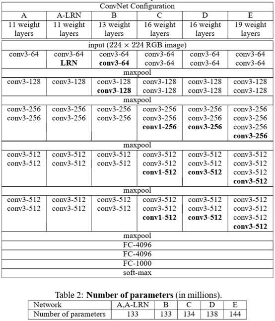
图1.4

　　加深结构都使用ReLU激活函数，VGG19比VGG16的区别在于多了3个卷积层，利用pytorch实现整VG16模型，VGG19同理。

 1 import torch as torch
 2 import torch.nn as nn
 3 
 4 class VGG16(nn.Module):
 5     def __init__(self,num_classes):
 6         super(VGG16,self).__init__()
 7         self.features = nn.Sequential(
 8             nn.Conv2d(3,64,kernel_size=3,padding=1),
 9             nn.ReLU(inplace=True),
10             nn.Conv2d(64,64,kernel_size=3,padding=1),
11             nn.ReLU(inplace=True),
12 
13             nn.Conv2d(64,128,kernel_size=3,padding=1),
14             nn.ReLU(inplace=True),
15             nn.Conv2d(128, 128, kernel_size=3, padding=1),
16             nn.ReLU(inplace=True),
17 
18             nn.Conv2d(128, 256, kernel_size=3, padding=1),
19             nn.ReLU(inplace=True),
20             nn.Conv2d(256, 256, kernel_size=3, padding=1),
21             nn.ReLU(inplace=True),
22             nn.Conv2d(256, 256, kernel_size=3, padding=1),
23             nn.ReLU(inplace=True),
24 
25             nn.Conv2d(256, 512, kernel_size=3, padding=1),
26             nn.ReLU(inplace=True),
27             nn.Conv2d(512, 512, kernel_size=3, padding=1),
28             nn.ReLU(inplace=True),
29             nn.Conv2d(512, 512, kernel_size=3, padding=1),
30             nn.ReLU(inplace=True),
31 
32             nn.Conv2d(512, 512, kernel_size=3, padding=1),
33             nn.ReLU(inplace=True),
34             nn.Conv2d(512, 512, kernel_size=3, padding=1),
35             nn.ReLU(inplace=True),
36             nn.Conv2d(512, 512, kernel_size=3, padding=1),
37             nn.ReLU(inplace=True)
38         )
39 
40         self.classifier = nn.Sequential(
41             nn.Linear(512*7*7,4096),
42             nn.ReLU(inplace=True),
43             nn.Dropout(),
44 
45             nn.Linear(4096,4096),
46             nn.ReLU(True),
47             nn.Dropout(),
48 
49             nn.Linear(4096,num_classes)
50         )
51     def forward(self, x):
52         x = self.features(x),
53         x = x.view(x.size(0),-1)
54         x = self.classifier(x)
55         return x

GoogLeNet

　　GoogLeNet专注于加深网络结构，与此同时引入了新的基本结构——Inception模块，从而来增加网络的宽度。GoogLeNet一共22层，它没有全连接层，在2014年的比赛中获得了冠军。

　　每个原始Inception模块由previous layer、并行处理层及filter concatenation层组成，如图1.5。并行处理层包含4个分支，即1*1卷积分支，3*3卷积分支，5*5卷积分支和3*3最大池化分支。一个关于原始Inception模块的最大问题是，5*5卷积分支即使采用中等规模的卷积核个数，在计算代价上也可能是无法承受的。这个问题在混合池化层之后会更为突出，很快的出现计算量的暴涨。

技术图片

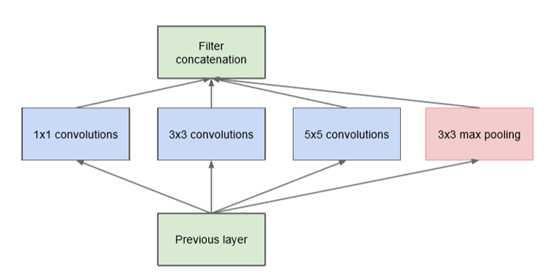
图1.5

　　为了克服原始Inception模块上的困难，GoogLeNet推出了一个新款，即采用1*1的卷积层来降低输入层的维度，使网络参数减少，因此减少网络的复杂性，如图1.6。因此得到降维Inception模块，称为inception V1。

技术图片

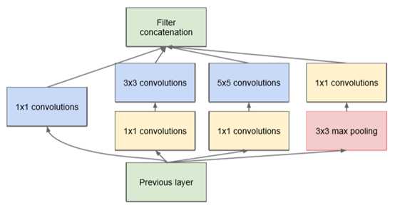
图1.6

　　从GoogLeNet中明显看出，共包含9个Inception V1模块，如图1.7所示。所有层均采用了ReLU激活函数。

　技术图片

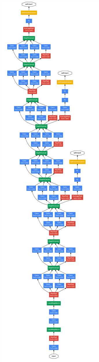
图1.7

　　自从2014年过后，Inception模块不断的改进，现在已发展到V4。GoogLeNet V2中的Inception参考VGGNet用两个3*3核的卷积层代替了具有5*5核的卷积层，与此同时减少了一个辅助分类器，并引入了Batch Normalization（BN），它是一个非常有用的正则化方法。V3相对于V2的学习效率提升了很多倍，并且训练时间大大缩短了。在ImageNet上的top-5错误率为4.8%。Inception V3通过改进V2得到，其核心思想是将一个较大的n*n的二维卷积拆成两个较小的一维卷积n*1和1*n。Inception V3有三种不同的结构（Base的大小分别为35*35、17*17、8*8），如图1.8所示，其中分支可能嵌套。GoogLeNet也只用了一个辅助分类器，在ImageNet上top-5的错误率为3.5%。Inception V4是一种与Inception V3类似或更复杂的网络模块。V4在ImageNet上top-5的错误率为3.08%。

技术图片

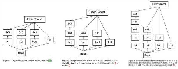
图1.8

　　接下来利用pytorch实现GoogLeNet中的Inception V2模块，其实整个GoogLeNet都是由Inception模块构成的。

 1 import torch.nn as nn
 2 import torch as torch
 3 import torch.nn.functional as F
 4 import torchvision.models.inception
 5 class BasicConv2d(nn.Module):
 6     def __init__(self,in_channels,out_channels,**kwargs):
 7         super(BasicConv2d,self).__init__()
 8         self.conv = nn.Conv2d(in_channels,out_channels,bias=False,**kwargs)
 9         self.bn = nn.BatchNorm2d(out_channels,eps=0.001)
10     def forward(self, x):
11         x = self.conv(x)
12         x = self.bn(x)
13         return F.relu(x,inplace=True)
14 
15 class Inception(nn.Module):
16     def __init__(self,in_channels,pool_features):
17         super(Inception,self).__init__()
18         self.branch1X1 = BasicConv2d(in_channels,64,kernel_size = 1)
19 
20         self.branch5X5_1 = BasicConv2d(in_channels,48,kernel_size = 1)
21         self.branch5X5_2 = BasicConv2d(48,64,kernel_size=5,padding = 2)
22 
23         self.branch3X3_1 = BasicConv2d(in_channels,64,kernel_size = 1)
24         self.branch3X3_2 = BasicConv2d(64,96,kernel_size = 3,padding = 1)
25         # self.branch3X3_2 = BasicConv2d(96, 96, kernel_size=1,padding = 1)
26 
27         self.branch_pool = BasicConv2d(in_channels,pool_features,kernel_size = 1)
28     def forward(self, x):
29         branch1X1 = self.branch1X1(x)
30 
31         branch5X5 = self.branch5X5_1(x)
32         branch5X5 = self.branch5X5_2(branch5X5)
33 
34         branch3X3 = self.branch3X3_1(x)
35         branch3X3 = self.branch3X3_2(branch3X3)
36 
37         branch_pool = F.avg_pool2d(x,kernel_size = 3,stride = 1,padding = 1)
38         branch_pool = self.branch_pool(branch_pool)
39 
40         outputs = [branch1X1,branch3X3,branch5X5,branch_pool]
41         return torch.cat(outputs,1)

ResNet

　　随着神经网络的深度不断的加深，梯度消失、梯度爆炸的问题会越来越严重，这也导致了神经网络的学习与训练变得越来越困难。有些网络在开始收敛时，可能出现退化问题，导致准确率很快达到饱和，出现层次越深、错误率反而越高的现象。让人惊讶的是，这不是过拟合的问题，仅仅是因为加深了网络。这便有了ResNet的设计，ResNet在2015年的ImageNet竞赛获得了冠军，由微软研究院提出，通过残差模块能够成功的训练高达152层深的网络，如图1.10所示。

ReNet与普通残差网络不同之处在于，引入了跨层连接（shorcut connection），来构造出了残差模块。

　　在一个残差模块中，一般跨层连接只有跨2~3层，如图1.9所示，但是不排除跨更多的层，跨一层的实验效果不理想。在去掉跨连接层，用其输出用H(x)，当加入跨连接层时，F(x) 与H(x)存在关系：F(x)：=H(x)-X，称为残差模块。既可以用全连接层构造残差模块，也可以用卷积层构造残差模块。基于残差模块的网络结构非常的深，其深度可达1000层以上。

技术图片

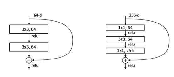
图1.9

技术图片

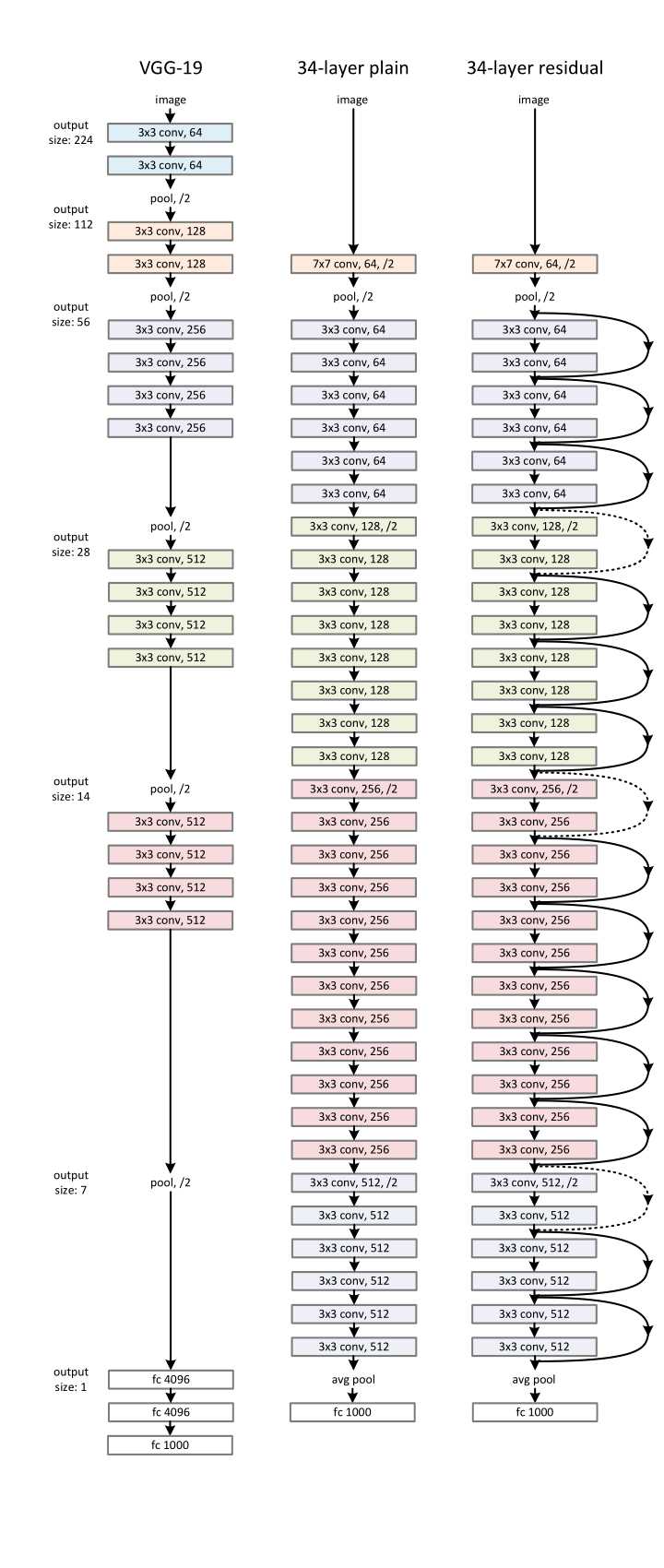
图1.10

　　用于ImageNet的5种深层残差网络结构，如图1.11所示。

技术图片

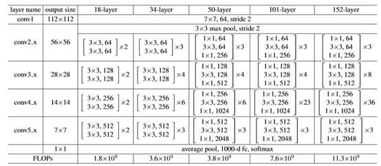
图1.11

　　从何凯明的论文中也读到plain-18、plain-34（即未加shotcut层）错误率比ResNet-18、ResNet-34（加了shotcut层）大了很多，如图1.12所示。

技术图片

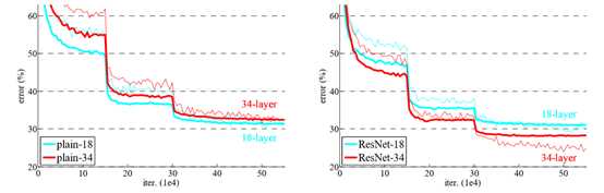
图1.12

　　下面利用pytorch实现ReNet的残差学习单元，此处参考了torchvision的model。

 1 import torch.nn as nn
 2 def conv3x3(in_planes, out_planes, stride=1):
 3     """3x3 convolution with padding"""
 4     return nn.Conv2d(in_planes, out_planes, kernel_size=3, stride=stride,
 5                      padding=1, bias=False)
 6 class BasicBlock(nn.Module):
 7     expansion = 1
 8     def __init__(self, inplanes, planes, stride=1, downsample=None):
 9         super(BasicBlock, self).__init__()
10         self.conv1 = conv3x3(inplanes, planes, stride)
11         self.bn1 = nn.BatchNorm2d(planes)
12         self.relu = nn.ReLU(inplace=True)
13         self.conv2 = conv3x3(planes, planes)
14         self.bn2 = nn.BatchNorm2d(planes)
15         self.downsample = downsample
16         self.stride = stride
17 
18     def forward(self, x):
19         residual = x
20         out = self.conv1(x)
21         out = self.bn1(out)
22         out = self.relu(out)
23         out = self.conv2(out)
24         out = self.bn2(out)
25         if self.downsample is not None:
26             residual = self.downsample(x)
27         out += residual
28         out = self.relu(out)
29         return out

当然，不管是LeNet，还是VGGNet，亦或是ResNet，这些经典的网络结构，pytorch的torchvision的model中都已经实现，并且还有预训练好的模型，可直接对模型进行微调便可使用。

Pytorch入门实战二：LeNet、AleNet、VGG、GoogLeNet、ResNet模型详解

标签：修改基于并行 ini 准确率 als challenge str 启动

原文地址：https://www.cnblogs.com/shenpings1314/p/10468418.html

踩

(0)

评论一句话评论（0）

分享档案

更多>

2021年07月29日 (22)
2021年07月28日 (40)
2021年07月27日 (32)
2021年07月26日 (79)
2021年07月23日 (29)
2021年07月22日 (30)
2021年07月21日 (42)
2021年07月20日 (16)
2021年07月19日 (90)
2021年07月16日 (35)

周排行