标签:target user nta code 思路 global listdir 决策 methods
数据集中的异常数据通常被成为异常点、离群点或孤立点等,典型特征是这些数据的特征或规则与大多数数据不一致,呈现出“异常”的特点,而检测这些数据的方法被称为异常检测。
异常数据根据原始数据集的不同可以分为离群点检测和新奇检测:
大多数情况我们定义的异常数据都属于离群点检测,对这些数据训练完之后再在新的数据集中寻找异常点。
所谓新奇检测是识别新的或未知数据模式和规律的检测方法,这些规律和只是在已有机器学习系统的训练集中没有被发掘出来。新奇检测的前提是已知训练数据集是“纯净”的,未被真正的“噪音”数据或真实的“离群点”污染,然后针对这些数据训练完成之后再对新的数据做训练以寻找新奇数据的模式。
新奇检测主要应用于新的模式、主题、趋势的探索和识别,包括信号处理、计算机视觉、模式识别、智能机器人等技术方向,应用领域例如潜在疾病的探索、新物种的发现、新传播主题的获取等。
新奇检测和异常检测有关,一开始的新奇点往往都以一种离群的方式出现在数据中,这种离群方式一般会被认为是离群点,因此二者的检测和识别模式非常类似。但是,当经过一段时间之后,新奇数据一旦被证实为正常模式,例如将新的疾病识别为一种普通疾病,那么新奇模式将被合并到正常模式之中,就不再属于异常点的范畴。
异常检测的适用场景:
注意点:
参考链接:
Python机器学习笔记 异常点检测算法——Isolation Forest
iForest 小结:
构造 iForest 的步骤如下:
获得 t个iTree之后,iForest训练就结束,然后我们可以用生成的iForest来评估测试数据了。对于一个训练数据X,我们令其遍历每一颗iTree,然后计算X 最终落在每个树第几层(X在树的高度)。然后我们可以得到X在每棵树的高度平均值,即 the average path length over t iTrees
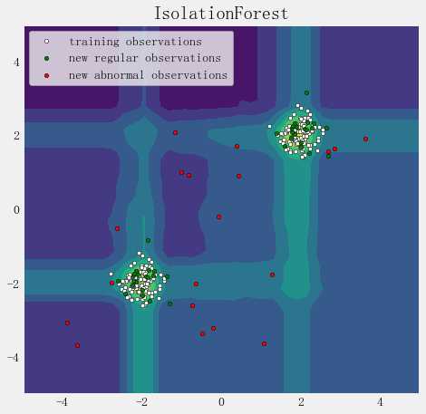
import numpy as np
import matplotlib.pyplot as plt
from sklearn.ensemble import IsolationForest

rng = np.random.RandomState(42)

# Generate  train data
X = 0.3 * rng.randn(100, 2)  #rng.uniform(0,1,(100,2))
X_train = np.r_[X + 2, X - 2]  #行拼接
X = 0.3 * rng.randn(20, 2)
X_test = np.r_[X + 2, X - 2]
X_outliers = rng.uniform(low=-4, high=4, size=(20, 2))

# fit the model
clf = IsolationForest(behaviour=‘new‘, max_samples=100, random_state=rng, contamination=‘auto‘)
clf.fit(X_train)

y_pred_train = clf.predict(X_train)
y_pred_test = clf.predict(X_outliers)

xx, yy = np.meshgrid(np.linspace(-5, 5, 50), np.linspace(-5, 5, 50))
Z = clf.decision_function(np.c_[xx.ravel(), yy.ravel()])
Z = Z.reshape(xx.shape)

plt.title("IsolationForest")
plt.contourf(xx, yy, Z)  #cmap=plt.cm.Blues_r
b1 = plt.scatter(X_train[:, 0], X_train[:, 1], c=‘white‘, s=20, edgecolor=‘k‘)
b2 = plt.scatter(X_test[:, 0], X_test[:, 1], c=‘green‘, s=20, edgecolor=‘k‘)
c = plt.scatter(X_outliers[:, 0], X_outliers[:, 1], c=‘red‘, s=20, edgecolor=‘k‘)
plt.axis(‘tight‘)
plt.xlim((-5, 5))
plt.ylim((-5, 5))
plt.legend([b1, b2, c],
           ["training observations", "new regular observations", "new abnormal observations"],
           loc="upper left")
plt.show()
OneClassSVM
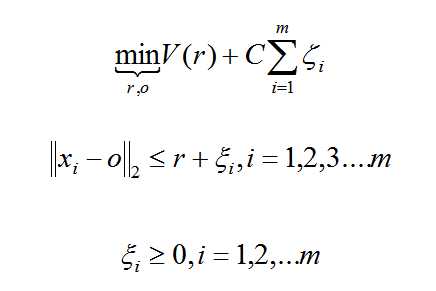
One Class Learning 比较经典的算法是One-Class-SVM,这个算法的思路非常简单,就是寻找一个超平面将样本中的正例圈出来,预测就是用这个超平面做决策,在圈内的样本就认为是正样本。由于核函数计算比较耗时,在海量数据的场景用的并不多;
严格来说,OneCLassSVM不是一种outlier detection,而是一种novelty detection方法:它的训练集不应该掺杂异常点,因为模型可能会去匹配这些异常点。但在数据维度很高,或者对相关数据分布没有任何假设的情况下,OneClassSVM也可以作为一种很好的outlier detection方法。
假设产生的超球体参数为中心 o 和对应的超球体半径 r >0,超球体体积V(r) 被最小化,中心 o 是支持行了的线性组合;跟传统SVM方法相似,可以要求所有训练数据点xi到中心的距离严格小于r。但是同时构造一个惩罚系数为 C 的松弛变量 ζi ,优化问题入下所示:
import numpy as np
import matplotlib.pyplot as plt
import matplotlib.font_manager
from sklearn import svm
# Generate train data
X = 0.3 * np.random.randn(100, 2)
X_train = np.r_[X + 2, X - 2]
X_test = np.r_[X + 2, X-2]
X_outliers = np.random.uniform(low=0.1, high=4, size=(20, 2))
#data = np.loadtxt(‘https://raw.githubusercontent.com/ffzs/dataset/master/outlier.txt‘, delimiter=‘ ‘)
#X_train = data[:900, :]
#X_test = data[-100:, :]
# 模型拟合
‘‘‘class sklearn.svm.OneClassSVM(kernel=‘rbf‘, degree=3, gamma=0.0, coef0=0.0,
tol=0.001, nu=0.5, shrinking=True, cache_size=200,
verbose=False, max_iter=-1, random_state=None)‘‘‘
clf = svm.OneClassSVM(nu=0.1, kernel=‘rbf‘, gamma=0.1)
clf.fit(X_train)
y_pred_train = clf.predict(X_train)
y_pred_test = clf.predict(X_test)
y_pred_outliers = clf.predict(X_outliers)
print ("novelty detection result:", y_pred_test)
n_error_train = y_pred_train[y_pred_train == -1].size
n_error_test = y_pred_test[y_pred_test == -1].size
n_error_outlier = y_pred_outliers[y_pred_outliers == 1].size
# plot the line , the points, and the nearest vectors to the plane
# 在平面中绘制点、线和距离平面最近的向量
#rand_mat = np.random.uniform(-1.0,1.0,(10000,5)) #np.random.randn(10000, 5)
#for i in range(X_train.shape[1]):
# rand_mat[:,i] = (rand_mat[:,i]-X_train[:,i].mean()) * X_train[:,i].std()
#rand_mat = pd.DataFrame(rand_mat, columns=list(‘abcde‘))
#rand_mat = rand_mat.sort_values(by = [‘a‘,‘b‘])
#rand_mat = rand_mat.values
#Z = clf.decision_function(rand_mat)
#xx = rand_mat[:,0].reshape((100,100))
#yy = rand_mat[:,1].reshape((100,100))
#xx, yy = np.meshgrid(np.linspace(X_train[:,0].min(), X_train[:,0].max(), 100),
# np.linspace(X_train[:,1].min(), X_train[:,1].max(), 100))
#Z = clf.decision_function(np.c_[xx.ravel(), yy.ravel(), X_train[np.random.randint(900,size=10000),2:]])
xx, yy = np.meshgrid(np.linspace(-5, 5, 500), np.linspace(-5, 5, 500))
Z = clf.decision_function(np.c_[xx.ravel(), yy.ravel()])
Z = Z.reshape(xx.shape)
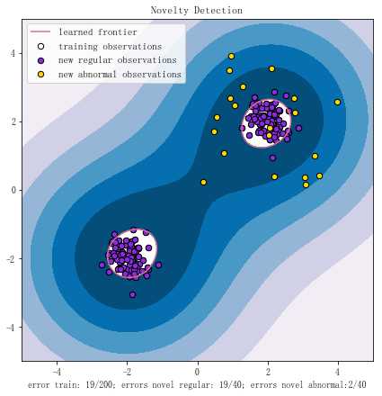
plt.title("Novelty Detection")
plt.contourf(xx, yy, Z, levels=np.linspace(Z.min(), 0, 7), cmap=plt.cm.PuBu)
a = plt.contour(xx, yy, Z, levels=[0, Z.max()], colors=‘palevioletred‘)
s = 40
b1 = plt.scatter(X_train[:, 0], X_train[:, 1], c=‘white‘, s=s, edgecolors=‘k‘)
b2 = plt.scatter(X_test[:, 0], X_test[:, 1], c=‘blueviolet‘, s=s, edgecolors=‘k‘)
c = plt.scatter(X_outliers[:, 0], X_outliers[:, 1], c=‘gold‘, s=s, edgecolors=‘k‘)
plt.axis(‘tight‘)
plt.xlim((-5, 5))
plt.ylim((-5, 5))
plt.legend([a.collections[0], b1, b2, c],
["learned frontier", ‘training observations‘, "new regular observations", "new abnormal observations"],
loc="upper left",
prop=matplotlib.font_manager.FontProperties(size=11))
plt.xlabel(
"error train: %d/200; errors novel regular: %d/40; errors novel abnormal:%d/40"%(
n_error_train, n_error_test, n_error_outlier) )
plt.show()
实际数据测试oneClassSVM
import numpy as np
import matplotlib.pyplot as plt
from numpy import genfromtxt
from sklearn import svm

#plt.style.use(‘fivethirtyeight‘)

def read_dataset(filePath, delimiter=‘,‘):
    return genfromtxt(filePath, delimiter=delimiter)

# use the same dataset
#tr_data = read_dataset(‘tr_data.csv‘)
tr_data = np.loadtxt(‘https://raw.githubusercontent.com/ffzs/dataset/master/outlier.txt‘, delimiter=‘ ‘)

‘‘‘
OneClassSVM(cache_size=200, coef0=0.0, degree=3, gamma=0.1, kernel=‘rbf‘,
      max_iter=-1, nu=0.05, random_state=None, shrinking=True, tol=0.001,
      verbose=False)
‘‘‘
clf = svm.OneClassSVM(nu=0.05, kernel=‘rbf‘, gamma=0.1)
clf.fit(tr_data[:,:2])
pred = clf.predict(tr_data[:,:2])

# inliers are labeled 1 , outliers are labeled -1
normal = tr_data[pred == 1]
abnormal = tr_data[pred == -1]

plt.plot(normal[:, 0], normal[:, 1], ‘bx‘)
plt.plot(abnormal[:, 0], abnormal[:, 1], ‘ro‘)
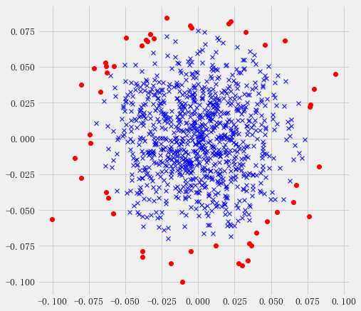
图片异常值检测OneClassSVM
import os
import cv2
from PIL import Image

def get_files(file_dir):
    for file in os.listdir(file_dir + ‘/AA475_B25‘):
       A.append(file_dir + ‘/AA475_B25/‘ + file)
    length_A = len(os.listdir(file_dir + ‘/AA475_B25‘))
    for file in range(length_A):
        img = Image.open(A[file])
        new_img = img.resize((128, 128))
        new_img = new_img.convert("L")
        matrix_img = np.asarray(new_img)
        AA.append(matrix_img.flatten())
    images1 = np.matrix(AA)
    return images1
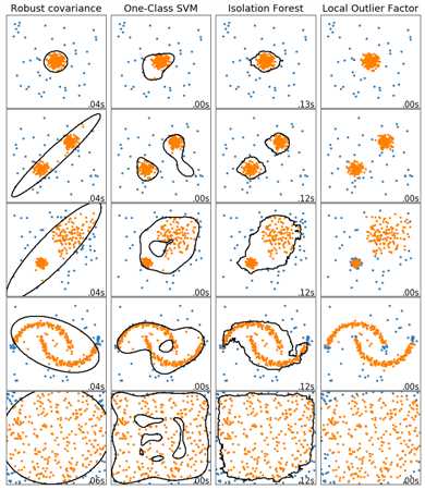
多种异常检测算法的比较
import time
import numpy as np
import matplotlib
import matplotlib.pyplot as plt
from sklearn import svm
from sklearn.datasets import make_blobs, make_moons
from sklearn.covariance import EllipticEnvelope
from sklearn.ensemble import IsolationForest
from sklearn.neighbors import LocalOutlierFactor

matplotlib.rcParams[‘contour.negative_linestyle‘] = ‘solid‘

# Example settings
n_samples = 300
outliers_fraction = 0.15
n_outliers = int(outliers_fraction * n_samples)
n_inliers = n_samples - n_outliers

# define outlier/ anomaly detection methods to be compared
anomaly_algorithms = [
    ("Robust covariance", EllipticEnvelope(contamination=outliers_fraction)),
    ("One-Class SVM", svm.OneClassSVM(nu=outliers_fraction, kernel=‘rbf‘,gamma=0.1)),
    ("Isolation Forest", IsolationForest(behaviour=‘new‘, contamination=outliers_fraction, random_state=42)),
    ("Local Outlier Factor", LocalOutlierFactor(n_neighbors=35, contamination=outliers_fraction))
]

# define datasets
blobs_params = dict(random_state=0, n_samples=n_inliers, n_features=2)
datasets = [
    make_blobs(centers=[[0, 0], [0, 0]], cluster_std=0.5, **blobs_params)[0],
    make_blobs(centers=[[2, 2], [-2, -2]], cluster_std=[0.5, 0.5], **blobs_params)[0],
    make_blobs(centers=[[2, 2], [-2, -2]], cluster_std=[1.5, 0.3], **blobs_params)[0],
    4. * (make_moons(n_samples=n_samples, noise=0.05, random_state=0)[0] - np.array([0.5, 0.25])),
    14. * (np.random.RandomState(42).rand(n_samples, 2) - 0.5)
]

# Compare given classifiers under given settings
xx, yy = np.meshgrid(np.linspace(-7, 7, 150), np.linspace(-7, 7, 150))

plt.figure(figsize=(len(anomaly_algorithms) * 2 + 3, 12.5))
plt.subplots_adjust(left=0.02, right=0.98, bottom=0.001, top=0.96, wspace=0.05, hspace=0.01)

plot_num = 1
rng = np.random.RandomState(42)


for i_dataset, X in enumerate(datasets):
    # add outliers
    X = np.concatenate([X, rng.uniform(low=-6, high=6, size=(n_outliers, 2))], axis=0)
    for name, algorithm in anomaly_algorithms:
        print(name , algorithm)
        t0 = time.time()
        algorithm.fit(X)
        t1 = time.time()
        plt.subplot(len(datasets), len(anomaly_algorithms), plot_num)
        if i_dataset == 0:
            plt.title(name, size=18)

        # fit the data and tag outliers
        if name == ‘Local Outlier Factor‘:
            y_pred = algorithm.fit_predict(X)
        else:
            y_pred = algorithm.fit(X).predict(X)

        # plot the levels lines and the points
        if name != "Local Outlier Factor":
            Z = algorithm.predict(np.c_[xx.ravel(), yy.ravel()])
            Z = Z.reshape(xx.shape)
            plt.contour(xx, yy, Z, levels=[0], linewidths=2, colors=‘black‘)

        colors = np.array(["#377eb8", ‘#ff7f00‘])
        plt.scatter(X[:, 0], X[:, 1], s=10, color=colors[(y_pred + 1) // 2])

        plt.xlim(-7, 7)
        plt.ylim(-7, 7)
        plt.xticks(())
        plt.yticks(())
        plt.text(0.99, 0.01, (‘%.2fs‘ % (t1 - t0)).lstrip(‘0‘),
                 transform=plt.gca().transAxes, size=15,
                 horizontalalignment=‘right‘)
        plot_num += 1

plt.show()
自编码器
如果我们只有正样本数据,没有负样本数据,或者说只关注学习正样本的规律,那么利用正样本训练一个自编码器,编码器就相当于单分类的模型,对全量数据进行预测时,通过比较输入层和输出层的相似度就可以判断记录是否属于正样本。由于自编码采用神经网络实现,可以用GPU来进行加速计算,因此比较适合海量数据的场景。
标签:target user nta code 思路 global listdir 决策 methods
原文地址:https://www.cnblogs.com/iupoint/p/11169029.html