标签:points htm between let work vol 角度 set sts
Let us take an analogy to explain the concept:
如果你想在某件事上做到更好,例如下棋,你会怎么做? 你或许会找一个比自己厉害的对手. 然后你会在你们对决中分析你错的地方和他对的地方, 并思考在下一场对决中你该如何击败对手.
你会不断重复这个过程,知道你击败对手. 这个理论同样适用于与我们训练一个好模型. So simply, for getting a powerful hero (viz generator), we need a more powerful opponent (viz discriminator)!
如下图所示,GAN 由两部分组成:Generator Neural Network and Discriminator Neural Network.
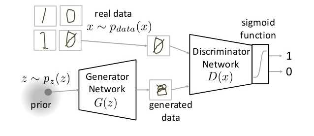
The Generator Network($G(z)$) 接受随机噪声输入($z$ from $p(z)$)来产生假样本($g$). 随后送入 Discriminator Network $D(x)$. Discriminator Network 的任务是判断 real data 和 fake data 的真假. It takes an input $x$ from $P_{data}(x)$ where $P_{data}(x)$ is ourreal data distribution. $D(x)$ then solvers a binary classification problem using sigmoid function giving outpit in the range 0 to 1.
Now the training of GAN is done (as we saw above) as a fight between generator and discriminator. This can be represented mathematically as:
\begin{equation}
\label{a}
\mathop{min}\limits_{G} \mathop{max}\limits_{D} V(D, G) \\
V(D, G) = E_{x \sim p_{data}(x)} [logD(x)] + E_{z \sim p_{z}(z)} [log(1-D(G(z))]
\end{equation}
train discriminator stage: 从判别器 $D$ 角度来看,它希望能尽可能区分出真假样本,即 maximize $V(D, G)$ to 0。具体来说,它一边希望 $D(x)$ 尽可能大,即 maximize $D(x)$ to 1. 另一边则希望 $D(G(z))$ 尽可能小,即 maximize $D(G(z))$ it to 0 (i.e. the log probability that the data from generated is fake is equal to 0).
train generator stage: 从生成器 $G$ 角度来看,它希望能够以假乱真 ,即 minimize the function $V$ to -NaN。 具体来说就是希望 $D(G(z))$ 尽可能大,即 maximize $D(G(x))$ to 1 (this stage only have second term).
Note: This method of training a GAN is taken from game theory called the minimax game.
So broadly a training phase has two main subparts and they are done sequentially:
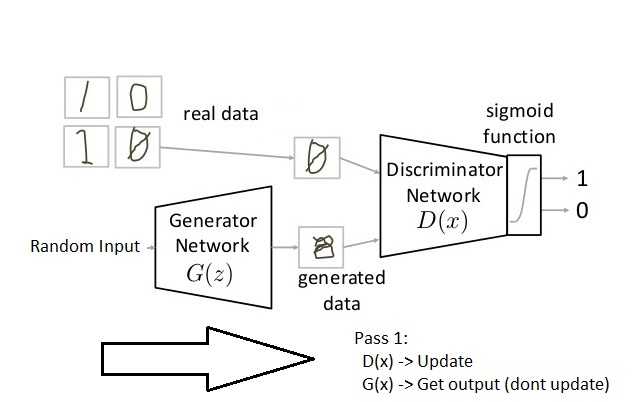
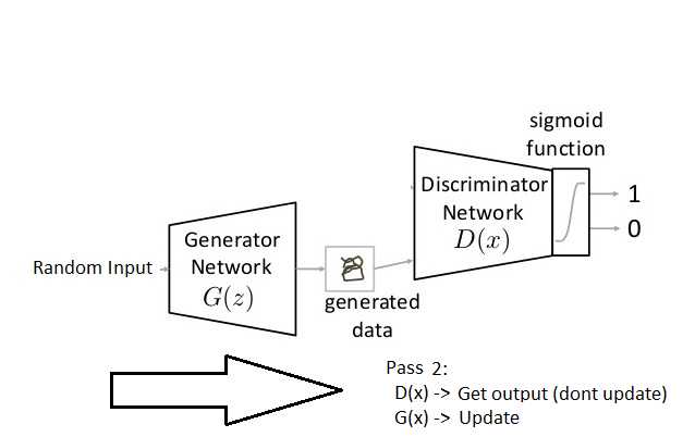
Step 1: Define the problem. Do you want to generate fake images or fake text. Here you should completely define the problem and collect data for it.
Step 2: Define architecture of GAN. Define how your GAN should look like. Should both your generator and discriminator be multi layer perceptrons, or convolutional neural networks? This step will depend on what problem you are trying to solve.
Step 3: Train Discriminator on real data for n epochs. Get the real data you want to generate fake on and train the discriminator to correctly predict them as real. Here value n can be any natural number between 1 and infinity.
Step 4: Generate fake inputs for generator and train Discriminator on fake data. Get generated data and let the discriminator correctly predict them as fake. (Step 3 and Step 4 are for Pass 1)
Step 5: Train Generator with the output of Discriminator. Now when the discriminator is trained, you can get its predictions and use it as an objective for training the generator. Train the generator to fool the discriminator. (This is Pass 2)
Step 6: Repeat step 3 to step 5 for a few epochs.
Step 7: Check if the fake data manually if it seems legit. If it seems appropriate, stop training, else go to step 3. This is a bit of a manual task, as hand evaluating the data is the best way to check the fakeness. When this step is over, you can evaluate whether the GAN is performing well enough.
You may ask, if we know what could these beautiful creatures (monsters?) do; why haven’t something happened? This is because we have barely scratched the surface. There’s so many roadblocks into building a “good enough” GAN and we haven’t cleared many of them yet. There’s a whole area of research out there just to find “how to train a GAN”
The most important roadblock while training a GAN is stability. If you start to train a GAN, and the discriminator part is much powerful that its generator counterpart, the generator would fail to train effectively. This will in turn affect training of your GAN. On the other hand, if the discriminator is too lenient; it would let literally any image be generated. And this will mean that your GAN is useless.
Another way to glance at stability of GAN is to look as a holistic convergence problem. Both generator and discriminator are fighting against each other to get one step ahead of the other. Also, they are dependent on each other for efficient training. If one of them fails, the whole system fails. So you have to make sure they don’t explode.
This is kind of like the shadow in Prince of Persia game . You have to defend yourself from the shadow, which tries to kill you. If you kill the shadow you die, but if you don’t do anything, you will definitely die!
There are other problems too, which I will list down here. (Reference: http://www.iangoodfellow.com/slides/2016-12-04-NIPS.pdf)
Note: Below mentioned images are generated by a GAN trained on ImageNet dataset.
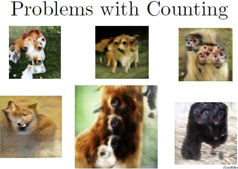
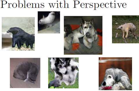
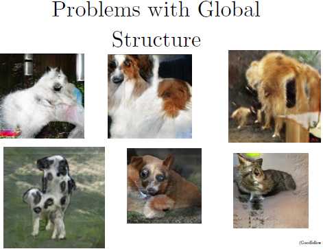
A substantial research is being done to take care of these problems. Newer types of models are proposed which give more accurate results than previous techniques, such as DCGAN, WassersteinGAN etc

import os
import torch
import torchvision
import torch.nn as nn
from torchvision import transforms
from torchvision.utils import save_image


# Device configuration
device = torch.device(‘cuda‘ if torch.cuda.is_available() else ‘cpu‘)
print(torch.__version__, device)

# Hyper-parameters
latent_size = 64
hidden_size = 256
image_size = 784
num_epochs = 200
batch_size = 100
sample_dir = ‘samples‘

# Create a directory if not exists
if not os.path.exists(sample_dir):
    os.makedirs(sample_dir)

# Image processing
transform = transforms.Compose([
                transforms.ToTensor(),
                transforms.Normalize(mean=(0.1307,),   # 3 for RGB channels
                                     std=(0.3081,))])

# MNIST dataset
mnist = torchvision.datasets.MNIST(root=‘H:/Other_DataSets/MNIST/‘,
                                   train=True,
                                   transform=transform,
                                   download=True)

# Data loader
data_loader = torch.utils.data.DataLoader(dataset=mnist,
                                          batch_size=batch_size,
                                          shuffle=True)

# Discriminator
D = nn.Sequential(
    nn.Linear(image_size, hidden_size),
    nn.LeakyReLU(0.2),
    nn.Linear(hidden_size, hidden_size),
    nn.LeakyReLU(0.2),
    nn.Linear(hidden_size, 1),
    nn.Sigmoid())

# Generator
G = nn.Sequential(
    nn.Linear(latent_size, hidden_size),
    nn.ReLU(),
    nn.Linear(hidden_size, hidden_size),
    nn.ReLU(),
    nn.Linear(hidden_size, image_size),
    nn.Tanh())

# Device setting
D = D.to(device)
G = G.to(device)

# Binary cross entropy loss and optimizer
criterion = nn.BCELoss()
d_optimizer = torch.optim.Adam(D.parameters(), lr=0.0002)
g_optimizer = torch.optim.Adam(G.parameters(), lr=0.0002)

def denorm(x):
    out = (x + 1) / 2
    return out.clamp(0, 1)

def reset_grad():
    d_optimizer.zero_grad()
    g_optimizer.zero_grad()

# Start training
total_step = len(data_loader)
for epoch in range(num_epochs):
    for i, (images, _) in enumerate(data_loader):
        images = images.reshape(batch_size, -1).to(device)

        # Create the labels which are later used as input for the BCE loss
        real_labels = torch.ones(batch_size, 1).to(device)
        fake_labels = torch.zeros(batch_size, 1).to(device)

        # ================================================================== #
        #                      Train the discriminator                       #
        # ================================================================== #

        # Compute BCE_Loss using real images where BCE_Loss(x, y): - y * log(D(x)) - (1-y) * log(1 - D(x))
        # Second term of the loss is always zero since real_labels == 1
        outputs = D(images)  # batch x 1
        d_loss_real = criterion(outputs, real_labels)
        real_score = outputs

        # Compute BCELoss using fake images
        # First term of the loss is always zero since fake_labels == 0
        z = torch.randn(batch_size, latent_size).to(device)
        fake_images = G(z) # batch x 784
        outputs = D(fake_images) # batch x 1
        d_loss_fake = criterion(outputs, fake_labels)
        fake_score = outputs

        # Backprop and optimize
        d_loss = d_loss_real + d_loss_fake
        reset_grad()
        d_loss.backward()
        d_optimizer.step()

        # ================================================================== #
        #                        Train the generator                         #
        # ================================================================== #

        # Compute loss with fake images
        z = torch.randn(batch_size, latent_size).to(device)
        fake_images = G(z) # batch x 784
        outputs = D(fake_images) # batch x 1

        # We train G to maximize log(D(G(z)) instead of minimizing log(1-D(G(z)))
        # For the reason, see the last paragraph of section 3. https://arxiv.org/pdf/1406.2661.pdf
        g_loss = criterion(outputs, real_labels)

        # Backprop and optimize
        reset_grad()
        g_loss.backward()
        g_optimizer.step()

        if (i+1) % 200 == 0:
            print(‘Epoch [{}/{}], Step [{}/{}], d_loss: {:.4f}, g_loss: {:.4f}, D(x): {:.2f}, D(G(z)): {:.2f}‘
                  .format(epoch, num_epochs, i+1, total_step, d_loss.item(), g_loss.item(),
                          real_score.mean().item(), fake_score.mean().item()))

    # Save real images
    if (epoch+1) == 1:
        images = images.reshape(images.size(0), 1, 28, 28)
        save_image(denorm(images), os.path.join(sample_dir, ‘real_images.png‘))

    # Save sampled images
    fake_images = fake_images.reshape(fake_images.size(0), 1, 28, 28)
    save_image(denorm(fake_images), os.path.join(sample_dir, ‘fake_images-{}.png‘.format(epoch+1)))

# Save the model checkpoints
torch.save(G.state_dict(), ‘G.ckpt‘)
torch.save(D.state_dict(), ‘D.ckpt‘)
We saw an overview of how these things work and got to know the challenges of training them. We will now see the cutting edge research that has been done using GANs
Increasing Resolution of an image
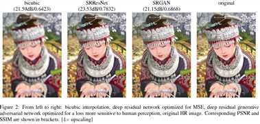

Link: https://github.com/junyanz/iGAN
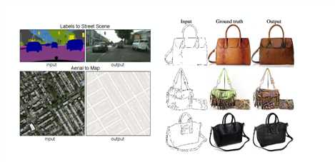
Paper: https://arxiv.org/pdf/1611.07004.pdf
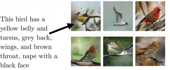
Paper : https://arxiv.org/pdf/1605.05396.pdf
Here are some resources which you might find helpful to get more in-depth on GAN
Phew! I hope you are now as excited about the future as I was when I first read about GANs. They are set to change what machines can do for us. Think of it – from preparing new recipes of food to creating drawings. The possibilities are endless.
In this article, I tried to cover a general overview of GAN and its applications. GAN is very exciting area and that’s why researchers are so excited about building generative models and you can see that new papers on GANs are coming out more frequently.
If you have any questions on GANs, please feel free to share them with me through comments.
GAN01: Introductory guide to Generative Adversarial Networks (GANs) and their promise!
标签:points htm between let work vol 角度 set sts
原文地址:https://www.cnblogs.com/xuanyuyt/p/11935900.html