标签:any dia 简化 eva gas control 输入 ase 指定
Published as a conference paper at ICLR 2018
Tero Karras、Timo Aila、Samuli Laine and Jaakko Lehtinen
NVIDIA and Aalto University
We describe a new training methodology for generative adversarial networks. The key idea is to grow both the generator and discriminator progressively: starting from a low resolution, we add new layers that model increasingly fine details as training progresses. This both speeds the training up and greatly stabilizes it, allowing us to produce images of unprecedented quality, e.g., CELEBA images at 10242. We also propose a simple way to increase the variation in generated im ages, and achieve a record inception score of 8.80 in unsupervised CIFAR10. Additionally, we describe several implementation details that are important for discouraging unhealthy competition between the generator and discriminator. Finally, we suggest a new metric for evaluating GAN results, both in terms of image quality and variation. As an additional contribution, we construct a higher-quality version of the CELEBA dataset.
我们为GAN描述了一个新的训练方法。方法的关键点就是渐进的让生成器和判别器都增长:从一个低分辨率开始,在训练过程中,我们不断添加新层使模型增加更好的细节。这个方法既加速了训练又使训练更加稳定,生成的图片质量史无前例的好,例如:1024*1024大小的CELEBA图片。我们也提出了一个简单的在生成图片的过程中增加变量的方法,并且在无监督数据集CIFAR10上获得了8.80分的记录。另外,我们描述了若干实现细节,这对打压生成器和判别器之间的非健康竞争是非常重要的。最后,我们提出了一种新的评估GAN结果的方法,包括图像质量和变化。因为增加项的贡献,我们构建了一个更高质量的CELEBA数据集版本。
Generative methods that produce novel samples from high-dimensional data distributions, such as images, are finding widespread use, for example in speech synthesis (van den Oord et al., 2016a), image-to-image translation (Zhu et al., 2017; Liu et al., 2017; Wang et al., 2017), and image inpainting (Iizuka et al., 2017). Currently the most prominent approaches are autoregressive models(van den Oord et al., 2016b;c), variational autoencoders (VAE) (Kingma & Welling, 2014), and generative adversarial networks (GAN) (Goodfellow et al., 2014). Currently they all have significant
strengths and weaknesses. Autoregressive models – such as PixelCNN – produce sharp images but are slow to evaluate and do not have a latent representation as they directly model the conditional distribution over pixels, potentially limiting their applicability. VAEs are easy to train but tend to produce blurry results due to restrictions in the model, although recent work is improving this (Kingma et al., 2016). GANs produce sharp images, albeit only in fairly small resolutions and with somewhat limited variation, and the training continues to be unstable despite recent progress (Salimans et al., 2016; Gulrajani et al., 2017; Berthelot et al., 2017; Kodali et al., 2017). Hybrid methods combine various strengths of the three, but so far lag behind GANs in image quality (Makhzani & Frey, 2017; Ulyanov et al., 2017; Dumoulin et al., 2016).
我们发现从高维度的数据分布中(例如图片)产生新颖样本的生成式方法正在广泛使用,例如语音合成(van den Oord et al., 2016a),图像到图像的转换(Zhu et al., 2017; Liu et al., 2017)以及图像绘制(Iizuka et al.,2017)。目前最好的方法是自动回归模型(van den Oord et al.,2016b;c),可变自动编码(VAE)(Kingma & Welling, 2014)以及GAN((Goodfellow et al., 2014)。目前他们都有显著的优势和劣势。自动回归模型–例如PixelCNN–会产生锐化的图片但是评估缓慢并且不具备一个潜在的代表性,因为他们是直接在像素上模型化条件分布,潜在的限制了他们的适用性。VAEs方法训练简单但是由于模型的限制倾向于产生模糊的结果,虽然最近的工作正在改善这个缺点(Kingma et al., 2016)。GANs方法虽然只能在相当小的分辨率并且带有一些限制的可变性分辨率上产生锐化图像,尽管最近有新的进展 (Salimans et al., 2016; Gulrajaniet al., 2017; Berthelot et al., 2017; Kodali et al., 2017)但是在训练上仍然是不稳定的。混合的方法结合了这三个方法的不同优点,但是目前在图片质量上仍然不如GANs(Makhzani & Frey, 2017; Ulyanov et al.,2017; Dumoulin et al., 2016)。
Typically, a GAN consists of two networks: generator and discriminator (aka critic). The generator produces a sample, e.g., an image, from a latent code, and the distribution of these images should ideally be indistinguishable from the training distribution. Since it is generally infeasible to engineer a function that tells whether that is the case, a discriminator network is trained to do the assessment, and since networks are differentiable, we also get a gradient we can use to steer both networks to the right direction. Typically, the generator is of main interest – the discriminator is an adaptive loss function that gets discarded once the generator has been trained.
典型的,一个GAN模型包括两个网络:生成式网络和判别式网络(aka critic)。生成式网络生成一个样本,例如:从一个潜在的代码中生成一副图片,这些生成的图片分布和训练的图片分布是不可分辨的。因为通过创建一个函数来辨别是生成样本还是训练样本一般是不可能的,所以一个判别器网络被训练去做这样一个评估,因为网络是可区分的,所以我们也可以得到一个梯度用来引导网络走到正确的方向。典型的,生成器是主要兴趣方–判别器就是一个适应性的损失函数,即一旦生成器被训练后,这个函数就要被丢弃。
There are multiple potential problems with this formulation. When we measure the distance between the training distribution and the generated distribution, the gradients can point to more or less random directions if the distributions do not have substantial overlap, i.e., are too easy to tell apart (Arjovsky & Bottou, 2017). Originally, Jensen-Shannon divergence was used as a distance metric (Goodfellow et al., 2014), and recently that formulation has been improved (Hjelm et al., 2017) and a number of more stable alternatives have been proposed, including least squares (Mao et al., 2016b), absolute deviation with margin (Zhao et al., 2017), and Wasserstein distance (Arjovsky et al., 2017; Gulrajani et al., 2017). Our contributions are largely orthogonal to this ongoing discussion, and we primarily use the improved Wasserstein loss, but also experiment with least-squares loss.
这个表述存在多种潜在的问题。例如:当我们测量训练分布和生成分布之间的距离时,如果分布之间没有大量的很容易分辨的重叠那么梯度可能指出或多或少的随机方向 (Arjovsky& Bottou, 2017)。原来, Jensen-Shannon散度被用作距离度量(Goodfellow et al., 2014),最近这个公式已经被改善(Hjelm et al., 2017)并且大量更多的可选方案被提出,包括least squares (Mao et al., 2016b),绝对边缘误差(absolute deviation with margin (Zhao et al., 2017)),以及Wasserstein 距离(Arjovsky et al., 2017; Gulrajani et al., 2017)。我们的贡献和目前正在进行的讨论大部分是正交的,并且我们基本使用改善的Wasserstein 损失,但是也有基于least-squares损失的实验。
The generation of high-resolution images is difficult because higher resolution makes it easier to tell the generated images apart from training images (Odena et al., 2017), thus drastically amplifying the gradient problem. Large resolutions also necessitate using smaller minibatches due to memory constraints, further compromising training stability. Our key insight is that we can grow both the generator and discriminator progressively, starting from easier low-resolution images, and add new layers that introduce higher-resolution details as the training progresses. This greatly speeds up training and improves stability in high resolutions, as we will discuss in Section 2.
高分辨率图片的生成是困难的因为更高的分辨率使得判别器更容易分辨是生成的图片还是训练图片(Odena et al., 2017),因此彻底放大了这个梯度问题。由于内存的限制,大分辨率使用更小的minibatches也是需要的,所以要和训练稳定性进行折中。我们的关键亮点在于我们可以同时渐进促进生产器和判别器增长,从比较简单的低分辨率开始,随着训练的发展,不断添加新的层引进更高分辨率细节。这个很大程度上加速了训练并且改善了在高分辨率图片上的稳定性,正如我们在Section 2中讨论的。
The GAN formulation does not explicitly require the entire training data distribution to be represented by the resulting generative model. The conventional wisdom has been that there is a tradeoff between image quality and variation, but that view has been recently challenged (Odena et al., 2017). The degree of preserved variation is currently receiving attention and various methods have been suggested for measuring it, including inception score (Salimans et al., 2016), multi-scale structural similarity (MS-SSIM) (Odena et al., 2017; Wang et al., 2003), birthday paradox (Arora & Zhang, 2017), and explicit tests for the number of discrete modes discovered (Metz et al., 2016). We will describe our method for encouraging variation in Section 3, and propose a new metric for evaluating the quality and variation in Section 5.
GAN公式没有明确要求所有的训练数据分布都由生成的生成式模型来表述。传统方法会在图片质量和可变性之间有一个折中,但是这个观点最近已经改变 (Odena et al., 2017)。保留的可变性的程度目前受到关注并且提出了多种方法去测量可变性,包括初始分数 (Salimans et al., 2016),多尺度结构相似性 (MS-SSIM) (Odena et al., 2017; Wang et al., 2003),生日悖论(Arora & Zhang,2017),以及发现的离散模式的显示测试 (Metz et al., 2016)。我们将在Section 3中描述我们鼓励可变性的方法,并在 Section 5中提出一个评估质量和可变性的新的度量。
Section 4.1 discusses a subtle modification to the initialization of networks, leading to a more balanced learning speed for different layers. Furthermore, we observe that mode collapses traditionally plaguing GANs tend to happen very quickly, over the course of a dozen minibatches. Commonly they start when the discriminator overshoots, leading to exaggerated gradients, and an unhealthy competition follows where the signal magnitudes escalate in both networks. We propose a mechanism to stop the generator from participating in such escalation, overcoming the issue (Section 4.2).
Section 4.1中对网络的初始化讨论了一个细小的修改,使得不同层的学习速度更加平衡。更进一步,我们观察到在十几个minibatches的过程中,GAN会更快速的发生令人讨厌的传统的模式崩塌现象,通常当判别器处理过度时模式崩塌开始,导致梯度过大,并且会在两个网络信号幅度增大的地方伴随着一个不健康的竞争。我们提出了一个机制去阻止生成器参与这样的升级,以克服这个问题 (Section 4.2)。
We evaluate our contributions using the CELEBA, LSUN, CIFAR10 datasets. We improve the best published inception score for CIFAR10. Since the datasets commonly used in benchmarking generative methods are limited to a fairly low resolution, we have also created a higher quality version of the CELEBA dataset that allows experimentation with output resolutions up to 1024 × 1024 pixels. This dataset and our full implementation are available at
https://github.com/tkarras/progressive_growing_of_gans, trained networks can be found at https://drive.google.com/open?id=0B4qLcYyJmiz0NHFULTdYc05lX0U along
我们使用CELEBA, LSUN, CIFAR10数据集去评估我们的贡献。对于 CIFAR10我们改善了已经公布的最好的初始分数。因为通常被用于评量标准的生成方法的数据集对于相当低的分辨率来说是受限制的,所以我们已经创建了一个更高质量版本的CELEBA数据集,允许输出分辨率高达 1024 × 1024像素的实验。我们正准备发布这个数据集。我们成果的全部实现在网址https://github.com/tkarras/progressive_growing_of_gans可以获得,带有结果图片的训练网络在 https://drive.google.com/open?id=0B4qLcYyJmiz0NHFULTdYc05lX0U 获得,补充的vidio说明数据集,额外的结果,隐藏的空间插值都在https://youtu.be/XOxxPcy5Gr4。
Our primary contribution is a training methodology for GANs where we start with low-resolution images, and then progressively increase the resolution by adding layers to the networks as visualized in Figure 1. This incremental nature allows the training to first discover large-scale structure of the image distribution and then shift attention to increasingly finer scale detail, instead of having to learn all scales simultaneously.
我们的主要贡献就是GANs的训练方法:从低分辨率图片开始,然后通过向网络中添加层逐渐的增加分辨率,正如Figure 1所示。这个增加的本质使得训练首先发现大尺度结构的图片分布,然后将关注点逐渐的转移到更好尺度细节上,而不是必须同时学习所有的尺度。
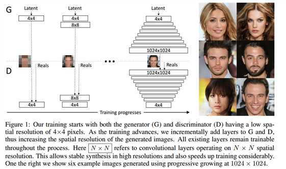
Figure1:我们的训练开始于有着一个4*4像素的低空间分辨率的生成器和判别器。随着训练的改善,我们逐渐的向生成器和判别器网络中添加层,因此增加生成图片的空间分辨率。所有现存的层通过进程保持可训练性。这里N×N是指卷积层在N×N的空间分辨率上进行操作。这个方法使得在高分辨率上稳定合成并且加快了训练速度。右图我们展示了六张通过使用在1024 × 1024空间分辨率上渐进增长的方法生成的样例图片。
We use generator and discriminator networks that are mirror images of each other and always grow in synchrony. All existing layers in both networks remain trainable throughout the training process. When new layers are added to the networks, we fade them in smoothly, as illustrated in Figure 2. This avoids sudden shocks to the already well-trained, smaller-resolution layers. Appendix A describes structure of the generator and discriminator in detail, along with other training parameters.
我们使用生成器网络和判别器网络作为相互的镜子并且同步促进两者的增长。同时在两个网络中的所有现存的层通过训练进程保持可训练性。当新的层被添加到网络中时,我们平滑的减弱它们,正如Fig2中所解释的。这样就避免了给已经训练好的更小分辨率的层带来突然的打击。附录A从细节上描述生成器网络和判别器网络的结构,并附有其他的训练参数。
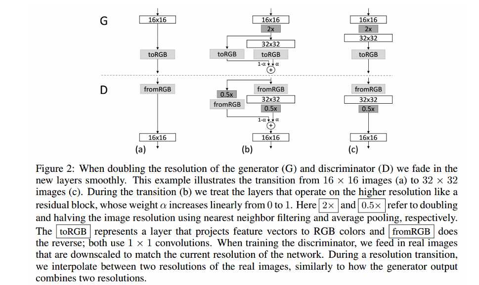
Figure 2:当把生成器和判别器的分辨率加倍时,我们会平滑的增强新的层。这个样例解释了如何从16 × 16像素的图片转换到32 × 32像素的图片。在转换(b)过程中,我们把在更高分辨率上操作的层视为一个残缺块,权重α从0到1线性增长。这里的2× 和 0.5× 指利用最近邻滤波和平均池化分别对图片分辨率加倍和折半。toRGB表示将一个层中的特征向量投射到RGB颜色空间中,fromRGB正好是相反的过程;这两个过程都是利用1 × 1卷积。当训练判别器时,我们插入下采样后的真实图片去匹配网络中的当前分辨率。在分辨率转换过程中,我们在两张真实图片的分辨率之间插值,类似于如何将两个分辨率结合到一起用生产器输出。
We observe that the progressive training has several benefits. Early on, the generation of smaller images is substantially more stable because there is less class information and fewer modes (Odena et al., 2017). By increasing the resolution little by little we are continuously asking a much simpler question compared to the end goal of discovering a mapping from latent vectors to e.g. 10242 images. This approach has conceptual similarity to recent work by Chen & Koltun (2017). In practice it stabilizes the training sufficiently for us to reliably synthesize megapixel-scale images using WGAN-GP loss (Gulrajani et al., 2017) and even LSGAN loss (Mao et al., 2016b).
Another benefit is the reduced training time. With progressively growing GANs most of the iterations are done at lower resolutions, and comparable result quality is often obtained up to 2–6 times faster, depending on the final output resolution.
我们观察到渐进训练有若干好处。早期,更小图像的生成非常稳定因为分类信息较少而且模式也少(Odena et al.,2017)。通过一点一点的增加分辨率,我们正不断的寻找一个更简单的问题,即:和最终目标进行比较,最终目标:从潜在向量中(例如1024*1024的图片)发现一个匹配。这个方法在概念上类似于最近Chen&Koltun(2017)的工作。在实践上,对于我们来说,它使训练充分稳点,因此在利用WGANGP损失(Gulrajani et al., 2017 )甚至LSGAN损失( Mao et al., 2016b)去合成megapixel-scale图片变得可靠。
另外一个好处是减少了训练时间。随着GANs网络的渐进增长,大部分的迭代都在较低分辨率下完成,对比结果质量加快了2-6倍的速度,这都依赖最后的输出分辨率。
The idea of growing GANs progressively is related to the work of Wang et al. (2017), who use multiple discriminators that operate on different spatial resolutions. That work in turn is motivated by Durugkar et al. (2016) who use one generator and multiple discriminators concurrently, and Ghosh et al. (2017) who do the opposite with multiple generators and one discriminator. Hierarchical GANs (Denton et al., 2015; Huang et al., 2016; Zhang et al., 2017) define a generator and discrimi nator for each level of an image pyramid. These methods build on the same observation as our work – that the complex mapping from latents to high-resolution images is easier to learn in steps – but the crucial difference is that we have only a single GAN instead of a hierarchy of them. In contrast to early work on adaptively growing networks, e.g., growing neural gas (Fritzke, 1995) and neuro evolution of augmenting topologies (Stanley & Miikkulainen, 2002) that grow networks greedily, we simply defer the introduction of pre-configured layers. In that sense our approach resembles layer-wise training of autoencoders (Bengio et al., 2007).
这个渐进增长的GANs想法是和课程GANs(他们使用多种不同空间分辨率的鉴别器)相关的,这个想法就是:把多个在不同空间分辨率上操作的判别器和一个单一的生成器连接,进一步的把调整两个分辨率之间的平衡作为训练时间的一个函数。这个想法按照两个方法轮流工作,即Durugkar et al. (2016)提出的同时使用一个生成器和多个判别器的方法以及Ghosh et al. (2017)提出的相反的使用多个生成器和一个判别器的方法。和早期的自适应增长型网络相比,例如:使网络贪婪增长的增长型神经气(Fritzke, 1995)以及增强型拓扑结构的神经进化(Stanley & Miikkulainen, 2002),我们简单的推迟了预配置层的介入。这种情况下,我们的方法和自动编码的智能层训练(Bengio et al., 2007)相像。
GANs have a tendency to capture only a subset of the variation found in training data, and Salimans et al. (2016) suggest "minibatch discrimination" as a solution. They compute feature statistics not only from individual images but also across the minibatch, thus encouraging the minibatches of generated and training images to show similar statistics. This is implemented by adding a minibatch layer towards the end of the discriminator, where the layer learns a large tensor that projects the input activation to an array of statistics. A separate set of statistics is produced for each example in a minibatch and it is concatenated to the layer‘s output, so that the discriminator can use the statistics internally. We simplify this approach drastically while also improving the variation.
抓取在训练数据中发现的变量的仅一个子集是GANs的一个趋势,Salimans et al. (2016)提出了"minibatch discrimination"作为解决方案。他们不仅从单个图片中而且还从小批量图片中计算特征统计,因此促进了生成的小批量图片和训练图片展示出了相似的统计。这是通过向判别器末端增加一个小批量层来实施,这个层学习一个大的张量将输入激活投射到一个统计数组中。在一个小批量中的每个样例会产生一个独立的统计集并且和输出层连接,以至于判别器可以从本质上使用这个统计。我们大大简化了这个方法同时提高了可变性。
Our simplified solution has neither learnable parameters nor new hyperparameters. We first compute the standard deviation for each feature in each spatial location over the minibatch. We then average these estimates over all features and spatial locations to arrive at a single value. We replicate the value and concatenate it to all spatial locations and over the minibatch, yielding one additional (constant) feature map. This layer could be inserted anywhere in the discriminator, but we have found it best to insert it towards the end (see Appendix A.1 for details). We experimented with a richer set of statistics, but were not able to improve the variation further. In parallel work, Lin et al. (2017) provide theoretical insights about the benefits of showing multiple images to the discriminator.
我们简化的解决方案既没有可学习的参数也没有新的超参数。我们首先计算基于小批量的每个空间位置的每个特征的标准偏差。然后对所有特征和空间位置的评估平均化到一个单一的值。我们复制这个值并且将它连接到所有空间位置以及小批量上,服从一个额外的(不变的)特征映射。这个层可以在网络中的任何地方插入,但是我们发现最好是插入到末端(see Appendix A.1 for details)。我们用一个丰富的统计集做实验,但是不能进一步提高可变性。
Alternative solutions to the variation problem include unrolling the discriminator (Metz et al., 2016) to regularize its updates, and a "repelling regularizer" (Zhao et al., 2017) that adds a new loss term to the generator, trying to encourage it to orthogonalize the feature vectors in a minibatch. The multiple generators of Ghosh et al. (2017) also serve a similar goal. We acknowledge that these solutions may increase the variation even more than our solution – or possibly be orthogonal to it – but leave a detailed comparison to a later time.
针对可变性这个问题另一个解决方案包括:展开判别器(Metz et al., 2016)去正则化它的更新,以及一个 "repelling regularizer" (Zhao et al., 2017)方法,即向生成器中添加一个新的损失项,尝试促进它与一个小批量中的特征向量正交化。Ghosh et al. (2017)提出的多个生成器也满足这样一个相似的目标。我们承认这些解决方案可能会增加可变性甚至比我们的解决方案更多–或者可能与它正交–但是后面留有一个细节性的比较。
GANs are prone to the escalation of signal magnitudes as a result of unhealthy competition between the two networks. Most if not all earlier solutions discourage this by using a variant of batch normalization (Ioffe & Szegedy, 2015; Salimans & Kingma, 2016; Ba et al., 2016) in the generator, and often also in the discriminator. These normalization methods were originally introduced to eliminate covariate shift. However, we have not observed that to be an issue in GANs, and thus believe that the actual need in GANs is constraining signal magnitudes and competition. We use a different approach that consists of two ingredients, neither of which include learnable parameters.
由于两个网络之间的不健康的一个竞争结果,GANs往往会有信号幅度升级情况。大多数早期的解决方案并不鼓励这种在生成器以及在判别器中使用批处理正则化的一个变量 (Ioffe & Szegedy, 2015; Salimans & Kingma, 2016; Ba et al., 2016)的方式。这些正则化方法原来是消除协变量偏移的。然而,我们没有观察到在GANs中存在这个问题,因此相信在GANs中需要的是制约信号幅度以及竞争问题。我们使用两个因素且都不包含可学习参数的不同方法。
We deviate from the current trend of careful weight initialization, and instead use a trivial N (0; 1) initialization and then explicitly scale the weights at runtime. To be precise, we set w^i = wi=c, where wi are the weights and c is the per-layer normalization constant from He‘s initializer (He et al., 2015). The benefit of doing this dynamically instead of during initialization is somewhat subtle, and relates to the scale-invariance in commonly used adaptive stochastic gradient descent methods such as RMSProp (Tieleman & Hinton, 2012) and Adam (Kingma & Ba, 2015). These
methods normalize a gradient update by its estimated standard deviation, thus making the update independent of the scale of the parameter. As a result, if some parameters have a larger dynamic range than others, they will take longer to adjust. This is a scenario modern initializers cause, and thus it is possible that a learning rate is both too large and too small at the same time. Our approach ensures that the dynamic range, and thus the learning speed, is the same for all weights. A similar reasoning was independently used by van Laarhoven (2017)
我们脱离了当前谨慎的权重初始化趋势,使用了一个数学上最简单的正太分布N (0; 1)初始化,然后在运行阶段显示缩放权重。为了更精确,我们设置这里写图片描述,wi是权重,c是来自于He等的初始化方法 (He et al., 2015)的前一层正则化常量。在初始化过程中动态做这种操作的好处是有一些微妙的,它关系到常规的使用自适应随机梯度下降法例如RMSProp (Tieleman & Hinton, 2012) 和 Adam (Kingma & Ba, 2015)方法保持的尺度不变性。这些方法通过评估标准差正则化一个梯度更新,因此使更新不依赖于参数的变化。结果,如果一些参数相比较其他参数而言有一个更大范围的动态变化,他们将花费更长的时间去调整。这是一个现在初始化问题面临的场景,因此有可能出现在同一时间学习速率既是最大值也是最小值的情况。我们的方法保证了动态范围,因此对于所有权重,学习速度都是一样 的。
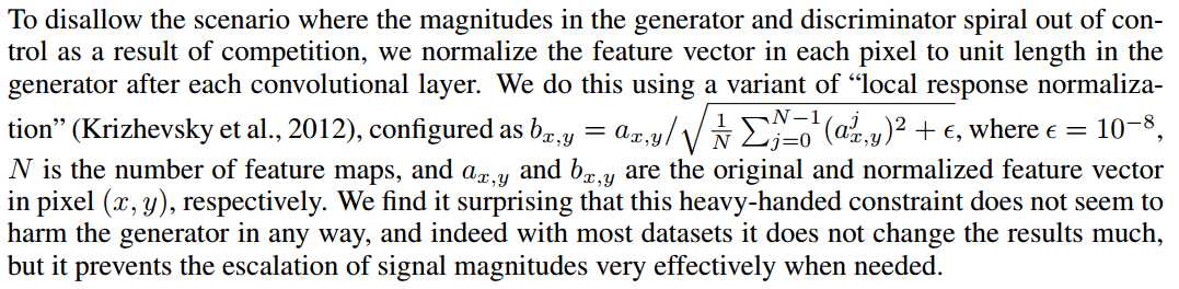
由于竞争的结果,为了防止出现在生成器和判别器中的量级逐渐脱离控制的场景,我们对每个像素中的特征向量进行归一化使每个卷积层之后的生成器中的长度可以单位化。我们只用一个"局部相应正则化" (Krizhevsky et al., 2012)变量,按照公式

这里写图片描述 配置,其中这里写图片描述 N表示特征匹配的数量,ax,y和bx,y分别表示像素(x,y)中的原始和归一化特征向量。我们惊喜的发现这个粗率的限制在任何方式下看起来都不会危害到这个生成器并且对于大多数数据集,它也不会改变太多结果,但是它却在有需要的时候有效的防止了信号幅度的增大。
In order to compare the results of one GAN to another, one needs to investigate a large number of images, which can be tedious, difficult, and subjective. Thus it is desirable to rely on automated methods that compute some indicative metric from large image collections. We noticed that existing methods such as MS-SSIM (Odena et al., 2017) find large-scale mode collapses reliably but fail to react to smaller effects such as loss of variation in colors or textures, and they also do not directly
assess image quality in terms of similarity to the training set.
为了把一个GAN的结果和另一个做比较,需要调查大量的图片,这可能是乏味的,困难的并且主观性的。因此依赖自动化方法–从大量的收集图片中计算一些指示性指标 是可取的。我们注意到现存的方法例如MS-SSIM (Odena et al., 2017)在发现大尺度模式的崩塌很可靠,但是对比较小的影响没有反应例如在颜色或者纹理上的损失变化,而且它们也不能直接对训练集相似的图片质量进行评估。
We build on the intuition that a successful generator will produce samples whose local image structure is similar to the training set over all scales. We propose to study this by considering the multiscale statistical similarity between distributions of local image patches drawn from Laplacian pyramid (Burt & Adelson, 1987) representations of generated and target images, starting at a low-pass resolution of 16 × 16 pixels. As per standard practice, the pyramid progressively doubles until the full resolution is reached, each successive level encoding the difference to an up-sampled version of the previous level.
我们的直觉是一个成功的生成器会基于所有尺度,产生局部图像结构和训练集是相似的样例。我们建议通过考虑两个分别来自于生成样例和目标图片的 Laplacian金字塔表示的局部图片匹配分布的多尺度统计相似性,并从 16 × 16像素的低通过分辨率开始,进行学习。随着每一个标准的训练,这个金字塔双倍的渐增直到获得全部分辨率,每个连续的水平的编码都不同于它先前的上采样版本。
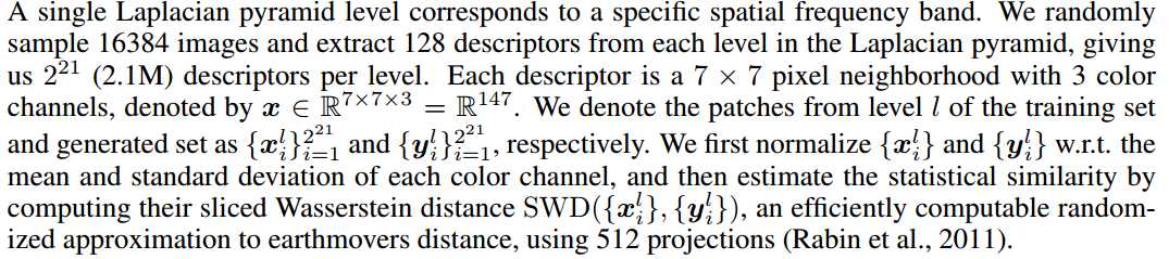
一个单一的拉普拉斯金字塔等级对应着一个特定空间频率带。我们随机采样16384 张图片并从拉普拉斯金字塔中的每一级中提取出128个描述符,每一级给我们2.1M描述符。每一个描述符都是带有3个颜色通道的 7 × 7相邻像素,通过
来指定。我们把训练集和生成集中的l级的匹配分别指定为
我们首先标准
述 w.r.t.每个颜色通道的均值和标准差,然后通过计算他们的
(sliced Wasserstein distance)值评估统计相似性,这是一种有效的使用512个映射 (Rabin et al., 2011)计算随机近似的EMD值(earthmovers distance)的方法。
Intuitively a small Wasserstein distance indicates that the distribution of the patches is similar, meaning that the training images and generator samples appear similar in both appearance and variation
at this spatial resolution. In particular, the distance between the patch sets extracted from the lowestresolution 16 × 16 images indicate similarity in large-scale image structures, while the finest-level
patches encode information about pixel-level attributes such as sharpness of edges and noise.
直观上,一个小的Wasserstein距离表示了块儿间的分布是相似的,意味着训练样例和生成样例在外貌以及空间分辨率的变化上都是相似的。特别是,从最低的分辨率 16 × 16的图片上提取出的块儿集之间的距离表明在大尺度图像结构方面是相似的,然而finest-level的块儿编码了关于像素级属性的信息例如边界的尖锐性和噪声。
In this section we discuss a set of experiments that we conducted to evaluate the quality of
our results. Please refer to Appendix A for detailed description of our network structures
and training configurations. We also invite the reader to consult the accompanying video
(https://youtu.be/G06dEcZ-QTg) for additional result images and latent space interpolations.
In this section we will distinguish between the network structure (e.g., convolutional layers, resizing), training configuration (various normalization layers, minibatch-related operations), and training loss (WGAN-GP, LSGAN).
这部分我们讨论了一系列的实验来评估我们结果的质量。我们的网络结构以及训练编译的细节描述请参考附件A。我们也邀请读着去参阅另外的结果图片的附带视频(https://youtu.be/XOxxPcy5Gr4) 以及隐藏的空间插值。这部分我们将区分网络结构 (e.g., convolutional layers, resizing),训练编译(不同的正则化层,相关的小批处理操作),以及训练损失 (WGAN-GP, LSGAN)。
We will first use the sliced Wasserstein distance (SWD) and multi-scale structural similarity (MSSSIM) (Odena et al., 2017) to evaluate the importance our individual contributions, and also perceptually validate the metrics themselves. We will do this by building on top of a previous state-of-theart loss function (WGAN-GP) and training configuration (Gulrajani et al., 2017) in an unsupervised setting using CELEBA (Liu et al., 2015) and LSUN BEDROOM (Yu et al., 2015) datasets in 128^2 resolution. CELEBA is particularly well suited for such comparison because the training images contain noticeable artifacts (aliasing, compression, blur) that are difficult for the generator to repro duce faithfully. In this test we amplify the differences between training configurations by choosing a relatively low-capacity network structure (Appendix A.2) and terminating the training once the dis
criminator has been shown a total of 10M real images. As such the results are not fully converged.
我们首先将使用SWD值和多尺度结构相似性(MSSSIM) (Odena et al., 2017) 去评估我们自己贡献的重要性,也从感知上验证度量本身。我们会在一个先前的最新损失函数 (WGAN-GP)的顶层进行编译并在一个128*128分辨率的 CELEBA (Liu et al., 2015)和LSUN BEDROOM (Yu et al., 2015)的非监督数据集上训练配置 (Gulrajani et al., 2017)。CELEBA 数据集特别适合这样的比较因为这些图片包含 了显著的伪迹(混叠,压缩,模糊),这些伪迹对于生成器来说重新准确的生成式很困难的。在这个测试中,我们通过选择一个相关的低容量网络结构(附件A.2)并且一旦判别器已经展示了总共10M的真实图片时就终止训练的方式来训练配置并放大训练配置间的差异。这样结果就不会全部相同(相似)。
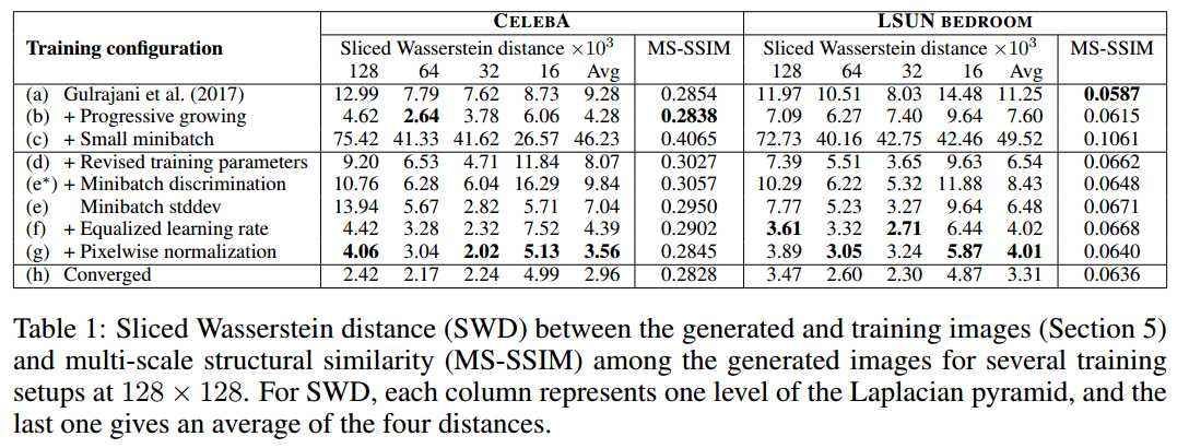
Table 1:生成样例和训练样例之间的SWD值( Sliced Wasserstein distance) (Section 5)和针对设置为 128 × 128分辨率的若干训练集的生成样例之间的多尺度结构相似性 (MS-SSIM)。对于SWD,每一列展示了拉普拉斯金字塔的一个层级,最后一列给出了苏哥距离的平均值。
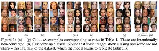
Figure 3: (a) – (g) CELEBA样例对应Table 1中的行。这些是有意不收敛的。(h)我们的收敛结果。注意有些图片是混叠的并且有些图片是非尖锐的–这是一个数据集的缺陷,这种模型会学习如实的复制。
Table 1 lists the numerical values for SWD and MS-SSIM in several training configurations, where our individual contributions are cumulatively enabled one by one on top of the baseline (Gulrajani et al., 2017). The MS-SSIM numbers were averaged from 10000 pairs of generated images, and SWD was calculated as described in Section 5. Generated CELEBA images from these configurations are shown in Figure 3. Due to space constraints, the figure shows only a small number of examples for each row of the table, but a significantly broader set is available in Appendix H. Intuitively, a good evaluation metric should reward plausible images that exhibit plenty of variation in
colors, textures, and viewpoints. However, this is not captured by MS-SSIM: we can immediately see that configuration (h) generates significantly better images than configuration (a), but MS-SSIM remains approximately unchanged because it measures only the variation between outputs, not similarity to the training set. SWD, on the other hand, does indicate a clear imp
Table 1列出了在若干训练配置中的SWD和MS-SSIM的数值,表明了我们的个人贡献逐渐的使基线的顶部(Gulrajani et al., 2017)一个接一个的成为可能。MS-SSIM个数是平均来自于10000对生成图片,SWD值计算在第5部分描述。Figure 3展示了来自于这些配置的生成的CELEBA图片。由于空间限制,这个图片仅仅展示了每行桌子的一小部分样例,但是在附近H中可以获得一个更广的集合。从直觉上说,一个好的评估标准应该奖励展示出的在颜色,纹理以及角度的大量变量中很相似的图片。然而,这并没有被MS-SSIM捕捉到:我们可以立刻看到配置(h)生成了比配置(a)更好的图片,但是MS-SSIM值保持近似不变因为它仅仅测量输出的变化而不测量输出与训练集的相似性。另一方面,SWD就有一个明显的改善。
The first training configuration (a) corresponds to Gulrajani et al. (2017), featuring batch normalization in the generator, layer normalization in the discriminator, and minibatch size of 64. (b) enables progressive growing of the networks, which results in sharper and more believable output images. SWD correctly finds the distribution of generated images to be more similar to the training set.
第一个训练配置(a)对应方法Gulrajani et al. (2017),特征化生成器中的批处理正则化,判别器中的层正则化,并且小批量大小为64。(b)能够使网络渐进增长,导致输出图片更加尖锐更加可信。SWD正确的发现了生成图片的分布于训练集更加相似。
Our primary goal is to enable high output resolutions, and this requires reducing the size of minibatches in order to stay within the available memory budget. We illustrate the ensuing challenges in (c) where we decrease the minibatch size from 64 to 16. The generated images are unnatural, which is clearly visible in both metrics. In (d), we stabilize the training process by adjusting the hyperparameters as well as by removing batch normalization and layer normalization (Appendix A.2). 我们的主要目标是输出高分辨率,这就要求减少小批量大小来保证运行在可获得的存储空间预算之内。在(c)中我们说明了将批处理有64降到16时遇到的挑战。在两个度量中可以清楚的看到生成的图片是不自然的。在(d)中,我们通过调整超参数以及移动批处理正则化和层正则化使训练进程稳定。
As an intermediate test (e∗), we enable minibatch discrimination (Salimans et al., 2016), which somewhat surprisingly fails to improve any of the metrics, including MS-SSIM that measures output variation. In contrast, our minibatch standard deviation (e) improves the average SWD scores and images. We then enable our remaining contributions in (f) and (g), leading to an overall improvement in SWD
and subjective visual quality. Finally, in (h) we use a non-crippled network and longer training – we feel the quality of the generated images is at least comparable to the best published results so far.
作为中间的一个测试(e∗),我们能够小批量的判别 (Salimans et al., 2016),有时也不能改善任何度量,包括测量输出变量的MS-SSIM值。相反,我们的小批量标准差 (e) 改善了SWD的平均得分还有图片。然后我们将我们的贡献用于 (f) 和(g)中,导致了在SWD以及主管视觉质量方面的总体改进。最后,在(h)中,我们使用一个非残疾网络以及更长时间的训练–我们认为生成图片的质量可以和目前最好的结果想媲美。
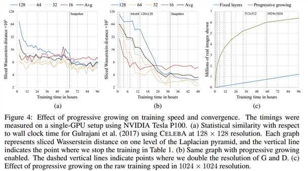
Figure 4: 在训练速度和收敛性方面渐进增长的影响。使用了一个NVIDIA Tesla P100 GPU测量时间。 (a) 关于Gulrajani et al. (2017)方法提到的挂钟,使用128 × 128分辨率的CELEBA数据集统计相似性。每个曲线都展示了拉普拉斯金字塔每一级的SWD值,垂直的线指示我们在Table 1中停止训练的点。(b)能够渐进增长的相同曲线。短的垂直线指示我们在G和D中双倍增加分别率的点。(c)在1024 × 1024分辨率以原训练速度渐进增长的影响。
Figure 4 illustrates the effect of progressive growing in terms of the SWD metric and raw image throughput. The first two plots correspond to the training configuration of Gulrajani et al. (2017) without and with progressive growing. We observe that the progressive variant offers two main benefits: it converges to a considerably better optimum and also reduces the total training time by about a factor of two. The improved convergence is explained by an implicit form of curriculum learning that is imposed by the gradually increasing network capacity. Without progressive growing, all layers of the generator and discriminator are tasked with simultaneously finding succinct intermediate representations for both the large-scale variation and the small-scale detail. With progressive growing, however, the existing low-resolution layers are likely to have already converged early on, so the networks are only tasked with refining the representations by increasingly smaller-scale effects as new layers are introduced. Indeed, we see in Figure 4(b) that the largest-scale statistical similarity curve (16) reaches its optimal value very quickly and remains consistent throughout the rest of the training. The smaller-scale curves (32, 64, 128) level off one by one as the resolution is increased, but the convergence of each curve is equally consistent. With non-progressive training in
Figure 4(a), each scale of the SWD metric converges roughly in unison, as could be expected.
Figure 4 说明了SWD度量的渐进增长的影响以及原始图像的吞吐率。前两个图对应Gulrajani et al. (2017)的带有和不带有渐进增长的训练配置。我们观察到渐进变量提供了两个主要优点:它收敛到一个非常好的最佳值并且总共的训练时间大概减少了一倍。改进的收敛值由课程学习的一个隐形格式来解释,这个课程学习有逐渐增长的网络容量决定。没有渐进增长情况下,生成器和判别器的所有层都要求同时找到简洁的大尺度变化和小尺度细节的中间展示。然而,渐进增长下,现存的低分辨率层可能在早期就已经收敛了,所以网络仅仅要求随着新层的加入,通过增加更小尺度影响得到更精炼的展示。确实,我们在Figure 4(b)中可以看到最大尺度的统计相似性曲线(16)很快的到达了它的优化值并且穿过训练的间断时间保持连续。更小尺度的曲线(32, 64, 128)随着分辨率的增加逐个的趋于平稳,但是每条曲线的收敛性是非常一致的。正如所料,非渐进训练的
The speedup from progressive growing increases as the output resolution grows. Figure 4(c) shows training progress, measured in number of real images shown to the discriminator, as a function of training time when the training progresses all the way to 10242 resolution. We see that progressive growing gains a significant head start because the networks are shallow and quick to evaluate at the beginning. Once the full resolution is reached, the image throughput is equal between the two methods. The plot shows that the progressive variant reaches approximately 6.4 million images in 96 hours, whereas it can be extrapolated that the non-progressive variant would take about 520 hours to reach the same point. In this case, the progressive growing offers roughly a 5:4× speedup.
Figure 4(a)中,每个SWD度量的收敛值尺度都是不平稳的。
To meaningfully demonstrate our results at high output resolutions, we need a sufficiently varied high-quality dataset. However, virtually all publicly available datasets previously used in GAN literature are limited to relatively low resolutions ranging from 322 to 4802. To this end, we created a high-quality version of the CELEBA dataset consisting of 30000 of the images at 1024 × 1024 resolution. We refer to Appendix C for further details about the generation of this dataset.
为了证明我们的结果是高输出分辨率,我们需要一个变化充分的高质量数据集。然而,以前在GaN文献中使用的几乎所有公开可用的数据集都局限于相对较低的从32*32 到480*480的分辨率范围。文中末尾,我们创建了一个高质量版本的CELEBA数据集,包含30000张1024 × 1024分辨率的图片。关于数据集生成的进一步细节参考附件C。
Our contributions allow us to deal with high output resolutions in a robust and efficient fashion. Figure 5 shows selected 1024 × 1024 images produced by our network. While megapixel GAN results have been shown before in another dataset (Marchesi, 2017), our results are vastly more varied and of higher perceptual quality. Please refer to Appendix F for a larger set of result images as well as the nearest neighbors found from the training data. The accompanying video shows latent space interpolations and visualizes the progressive training. The interpolation works so that we first randomize a latent code for each frame (512 components sampled individually from N (0; 1)), then blur the latents across time with a Gaussian (σ = 45 frames @ 60Hz), and finally normalize each vector to lie on a hypersphere.
我们的贡献允许我们以一个稳健高效的方式处理高分辨率的输出。Figure 5选择了我们的网络生成的1024 × 1024分辨的图片。然而在另一个数据集上 (Marchesi, 2017),兆像素的GAN结果已经在这之前展示出来了,但我们的结果更加多样化,感知质量也更高。一个更大的结果图像集以及从训练数据中找到的最近邻图像集请参考附件F。附带的视频显示了潜在的空间插值和可视化的循序渐进的训练。插值使我们首先随机化一个每一帧的潜在编码(来自于正太分布N (0; 1)的512个独立的样例组件),然后我们用一个高斯函数 (σ = 45 frames @ 60Hz)跨越时间模糊化潜在特征,最后归一化每个向量到一个单位超球面上。
We trained the network on 8 Tesla V100 GPUs for 4 days, after which we no longer observed qualitative differences between the results of consecutive training iterations. Our implementation used an adaptive minibatch size depending on the current output resolution so that the available memory budget was optimally utilized.
我们在一块NVIDIA Tesla P100 GPU上训练了20天的网络,直到我们观察不到连续的训练迭代结果之间的质量差异。我们的实施方法被用在一个依赖于当前输出分辨率的自适应小批量大小的网络上使可获得的内存预算被最佳利用。
In order to demonstrate that our contributions are largely orthogonal to the choice of a loss function, we also trained the same network using LSGAN loss instead of WGAN-GP loss. Figure 1 shows six examples of 10242 images produced using our method using LSGAN. Further details of this setup are given in Appendix B.
为了证明我们的贡献在很大程度上和损失函数的选择是正交的,我们也使用 LSGAN 损失来替代WGAN-GP损失训练 了相同的网络。Figure 1展示了使用我们方法和使用 LSGAN方法产生的 1024*1024分辨率的图片中的六个样例,设置的详细细节在附件B中给出。
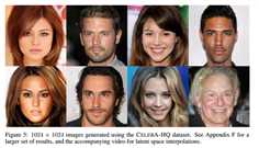
Figure 5:使用CELEBA-HQ 数据集生成的1024 × 1024分辨率的图片。附件F有更大的结果集,以及潜在空间插值的附带视频。右边,是由Marchesi (2017) 提出的一个更早期的兆像素GAN生成的两幅图片,展示限制的细节以及变化。
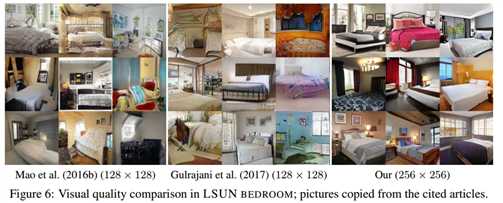
Figure 6:在 LSUN BEDROOM数据集上的可视化质量比较;图片复制于引用的文章。
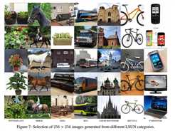
Figure 6 shows a purely visual comparison between our solution and earlier results in LSUN BEDROOM. Figure 7 gives selected examples from seven very different LSUN categories at 2562. A larger, non-curated set of results from all 30 LSUN categories is available in Appendix G, and the video demonstrates interpolations. We are not aware of earlier results in most of these categories, and while some categories work better than others, we feel that the overall quality is high.
Figure 6展示了一个纯粹的我们的解决方案和在 LSUN BEDROOM数据集上的早期结果的视觉比较。Figure 7给了被选择的7个不同的LSUN种类的256*256分辨率的样例。附件G中可以获得一个更大的,没有组织的所有30个LSUN种类的结果集,视频证明插值。我们不知道这些种类的早期结果,虽然有些种类比其它的要好,但是我们感觉整体质量是高的。
The best inception scores for CIFAR10 (10 categories of 32 × 32 RGB images) we are aware of are 7.90 for unsupervised and 8.87 for label conditioned setups (Grinblat et al., 2017). The large difference between the two numbers is primarily caused by "ghosts" that necessarily appear between classes in the unsupervised setting, while label conditioning can remove many such transitions.
我们知道的CIFAR10(10 categories of 32 × 32 RGB images) 的最好初始得分是:非监督数据集7.9分,带标签条件设置的数据集8.87分(Grinblat et al., 2017)。这两个数字之间的最大差异主要是由 "ghosts"导致的,在非监督环境中它必然出现在类之间,然而在有标签条件时可以移除很多这样的转换。
当我们的所有贡献都成功的时候,我们在非监督环境中会有8.8的得分。附录D显示了一组有代表性的结果图像,以及从早期方法得到的更全面的结果列表。网络和训练设置对CELEBA数据集要求是一样的,当然进程限制为32*32分辨率。仅有的用户化就是WGAN-GP的正则化项
Gulrajani et al. (2017)使用γ = 1.0,对应1-Lipschitz,但是我们注意到事实上最小化ghosts会使转换 (γ = 750)更好更快。我们还没有用其他数据集尝试这个方法。
While the quality of our results is generally high compared to earlier work on GANs, and the training is stable in large resolutions, there is a long way to true photorealism. Semantic sensibility and understanding dataset-dependent constraints, such as certain objects being straight rather than curved, leaves a lot to be desired. There is also room for improvement in the micro-structure of the images. That said, we feel that convincing realism may now be within reach, especially in CELEBA-HQ.
我们的结果质量普遍高于先前的在GANs上的质量,并且在大分辨率上的训练稳定,对于真正的真实照片来说还有好长的路。对依赖数据的限制的语义敏感性和理解还有很多需要提高,例如确定的目标是直接可得的而不是间接得到的。图像的微观结构还有改进的余地。就是说,我们觉得 convincing realism现在是可能实现的,特别是CELEBA-HQ。
附件:
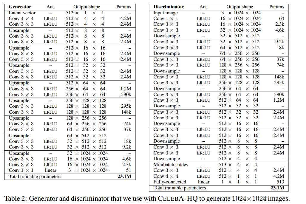
Table 2 shows network architectures of the full-resolution generator and discriminator that we use with the CELEBA-HQ dataset. Both networks consist mainly of replicated 3-layer blocks that we introduce one by one during the course of the training. The last Conv 1 × 1 layer of the generator corresponds to the toRGB block in Figure 2, and the first Conv 1 × 1 layer of the discriminator similarly corresponds to fromRGB. We start with 4 × 4 resolution and train the networks until we have shown the discriminator 800k real images in total. We then alternate between two phases: fade in the first 3-layer block during the next 800k images, stabilize the networks for 800k images, fade in the next 3-layer block during 800k images, etc.
表 2 显示了我们用于 CELEBA-HQ 数据集的全分辨率生成器和鉴别器的网络体系结构。两个网络主要由复制的 3 层模块组成,在培训过程中我们逐个介绍的这些块。生成器的最后一个 Conv 1 × 1 层对应于图 2 中的 toRGB 块,而第一个 Conv 1 ×1 层的鉴别器同样对应于 fromRGB。我们从 4 × 4 分辨率开始,并训练网络,直到我们总共显示了 800k 真实图像的鉴别器。然后,我们在两个阶段之间交替:在接下来的 800k 图像中在第一个 3 层块中淡入淡出,稳定 800k 图像的网络,在 800k 图像期间在下一个 3 层块中淡入淡出,等等。
Our latent vectors correspond to random points on a 512-dimensional hypersphere, and we represent training and generated images in [-1,1]. We use leaky ReLU with leakiness 0.2 in all layers of both networks, except for the last layer that uses linear activation. We do not employ batch normalization, layer normalization, or weight normalization in either network, but we perform pixelwise normalization of the feature vectors after each Conv 3×3 layer in the generator as described in Section 4.2. We initialize all bias parameters to zero and all weights according to the normal distribution with unit variance. However, we scale the weights with a layer-specific constant at runtime as described in Section 4.1. We inject the across-minibatch standard deviation as an additional feature map at 4 × 4 resolution toward the end of the discriminator as described in Section 3. The upsampling and downsampling operations in Table 2 correspond to 2 × 2 element replication and average pooling, respectively.
我们的潜在向量对应于 512 维超球上的随机点,我们在 [-1,1] 中表示训练和生成的图像。我们在两个网络的所有层中使用leakiness 0.2 的leaky ReLU,但最后一个使用线性激活的层除外。我们未在任一网络中采用批处理规范化、层规范化或权重规范化,但我们在生成器中的每个 Conv 3×3 层后按像素对要素矢量执行像素规范化,如第 4.2 节所述。我们根据单位方差的正态分布将所有偏置参数初始化为零和所有权重。但是,我们使用运行时的特定于图层的常量缩放权重,如第 4.1 节所述。我们将跨小批量标准差注入到附加要素图中,分辨率为 4 × 4,接近第 3 节所述的鉴别器末端。表 2 中的上采样和向下采样操作分别对应于 2 × 2 元素复制和平均池。
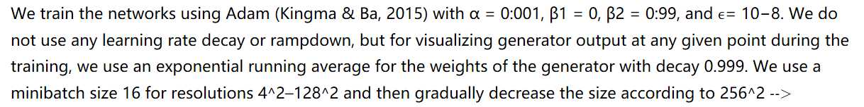
14, 512^2 -->6, and 1024^2--->3 to avoid exceeding the available memory budget. We use the WGAN-GP loss, but unlike Gulrajani et al. (2017), we alternate between optimizing the generator and discriminator on a per-minibatch basis, i.e., we set ncritic = 1. Additionally, we introduce a fourth term into the discriminator loss with an extremely small weight to keep the discriminator output from drifting too far away from zero. To be precise,

我们使用 Adam (Kingma & Ba, 2015) 训练网络,α = 0:001, β1 = 0, β2 = 0:99,? = 10+8。我们不使用任何学习速率衰减或降速,但为了在训练期间在任意给定点可视化发生成输出,我们使用衰减 0.999 的生成器权重的指数运行平均值。我们使用迷你批量大小 16 分辨率 4^2–128^2,然后根据256^2 --> 14, 512^2 --> 6, and 1024^2---> 3
以避免超出可用内存预算。我们使用 WGAN-GP 损耗,但与 Gulrajani 等人 (2017) 不同,我们根据每个小批量优化生成器和判别器(即,我们设置 ncritic = 1)之间交替。此外,我们引入第四个术语到鉴别器损失与极小的权重,以防止鉴别器输出漂移太远从零。确切地说

Whenever we need to operate on a spatial resolution lower than 1024 × 1024, we do that by leaving out an appropriate number copies of the replicated 3-layer block in both networks. Furthermore, Section 6.1 uses a slightly lower-capacity version, where we halve the number of feature maps in Conv 3 × 3 layers at the 16 × 16 resolution, and divide by 4 in the subsequent resolutions. This leaves 32 feature maps to the last Conv 3 × 3 layers. In Table 1 and Figure 4 we train each resolution for a total 600k images instead of 800k, and also fade in new layers for the duration of 600k images.
每当我们需要对低于 1024 × 1024 的空间分辨率进行操作时,我们会通过在两个网络中保留复制的 3 层块的适当数量副本来执行此操作。此外,第 6.1 节使用稍低的容量版本,其中我们将 Conv 3 + 3 层中的要素映射数在 16 × 16 分辨率下减半,并在后续分辨率中除以 4。这将留下 32 个要素映射到最后一个 Conv 3 + 3 图层。在表 1 和图 4 中,我们针对总共 600k 图像(而不是 800k)训练每个分辨率,并在 600k 图像的持续期间在新图层中淡入淡出。
For the "Gulrajani et al. (2017)" case in Table 1, we follow their training configuration as closely as possible. In particular, we set α = 0:0001, β2 = 0:9, ncritic = 5, drift = 0, and minibatch size 64. We disable progressive resolution, minibatch stddev, as well as weight scaling at runtime, and initialize all weights using He‘s initializer (He et al., 2015). Furthermore, we modify the generator by replacing LReLU with ReLU, linear activation with tanh in the last layer, and pixelwise normalization with batch normalization. In the discriminator, we add layer normalization to all Conv 3 × 3 and Conv 4 × 4 layers. For the latent vectors, we use 128 components sampled independently from the normal distribution.
对于表 1 中的"Gulrajani 等人(2017)"案例,我们尽可能密切地关注他们的培训配置。特别是,我们设置 #= 0:0001,^2 = 0:9,ncritic = 5,漂移 = 0,和微型批处理大小 64。我们禁用渐进式分辨率、微型批处理 stddev 以及在运行时缩放权重,并使用 He 的初始化器初始化所有权重(He 等人,2015 年)。此外,我们修改了生成器,将 LReLU 替换为 ReLU,在最后一层用 tanh 进行线性激活,并用批处理规范化进行像素规范化。在鉴别器中,我们将层规范化添加到所有 Conv 3 + 3 和 Conv 4 = 4 层。对于潜在向量,我们使用独立于正态分布采样的 128 个分量。
We find that LSGAN is generally a less stable loss function than WGAN-GP, and it also has a tendency to lose some of the variation towards the end of long runs. Thus we prefer WGAN-GP, but have also produced high-resolution images by building on top of LSGAN. For example, the 1024^2 images in Figure 1 are LSGAN-based.
1024×1024的B最小二乘GAN(LSGAN)
我们发现LSGAN通常是一个比WGAN-GP更不稳定的损失函数,并且在长期运行结束时也有失去一些变化的趋势。因此,我们更喜欢WGAN-GP,但也通过在LSGAN上构建来生成解决方案图像。例如,图片1的1024^2图像基于Lsgan
On top of the techniques described in Sections 2–4, we need one additional hack with LSGAN that prevents the training from spiraling out of control when the dataset is too easy for the discriminator, and the discriminator gradients are at risk of becoming meaningless as a result. We adaptively increase the magnitude of multiplicative Gaussian noise in discriminator as a function of the discriminator‘s output. The noise is applied to the input of each Conv 3 × 3 and Conv 4 × 4 layer. There is a long history of adding noise to the discriminator, and it is generally detrimental for the image quality (Arjovsky et al., 2017) and ideally one would never have to do that, which according to our tests is the case for WGAN-GP (Gulrajani et al., 2017). The magnitude of noise is determined as

is an exponential moving average of the discriminator output d. The motivation behind this hack is that LSGAN is seriously unstable when d approaches (or exceeds) 1:0.
除了第2-4节中描述的技术外,我们还需要使用LSGAN进行一次额外的破解,以防止当数据集对鉴别器太容易时训练失控,并且鉴别器半径有可能因此变得毫无意义。我们适当地增大判别器中增加高斯噪声的用于判别器的输出。噪声应用于输入oeach Conv 3 x 3和Conv 4 x 4层。在鉴别器中添加噪声的历史很长,它通常有损图像质量(Arjovsky等人,2017年),理想情况下,人们不会这样做,根据我们的测试,WGAN-GP就是这样(Gullajani等人,2017年)。噪声的大小被确定为

它是判别器输出d的指数移动平均值,此攻击的动机是当d接近(或超过)1:0时LSGAN是不稳定的
中文翻译:
https://blog.csdn.net/liujunru2013/article/details/78545882
【GAN论文-01】翻译-Progressive growing of GANS for improved quality ,stability,and variation-论文
标签:any dia 简化 eva gas control 输入 ase 指定
原文地址:https://www.cnblogs.com/yifanrensheng/p/12989824.html