标签:des style blog http ar io os sp for
Consider a supervised learning problem where we have access to labeled training examples (x(i),y(i)). Neural networks give a way of defining a complex, non-linear form of hypotheses hW,b(x), with parameters W,b that we can fit to our data.
To describe neural networks, we will begin by describing the simplest possible neural network, one which comprises a single "neuron." We will use the following diagram to denote a single neuron:

This "neuron" is a computational unit that takes as input x1,x2,x3 (and a +1 intercept term), and outputs  , where
  is called the activation function. In these notes, we will choose
  to be the sigmoid function:
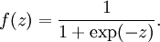
Thus, our single neuron corresponds exactly to the input-output mapping defined by logistic regression.
Although these notes will use the sigmoid function, it is worth noting that another common choice for f is the hyperbolic tangent, or tanh, function:
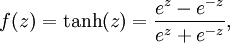
Here are plots of the sigmoid and tanh functions:


The tanh(z) function is a rescaled version of the sigmoid, and its output range is [ − 1,1] instead of [0,1].
Note that unlike some other venues (including the OpenClassroom videos, and parts of CS229), we are not using the convention here of x0 = 1. Instead, the intercept term is handled separately by the parameter b.
Finally, one identity that‘ll be useful later: If f(z) = 1 / (1 + exp( − z)) is the sigmoid function, then its derivative is given by f‘(z) = f(z)(1 − f(z)). (If f is the tanh function, then its derivative is given by f‘(z) = 1 − (f(z))2.) You can derive this yourself using the definition of the sigmoid (or tanh) function.
A neural network is put together by hooking together many of our simple "neurons," so that the output of a neuron can be the input of another. For example, here is a small neural network:

In this figure, we have used circles to also denote the inputs to the network. The circles labeled "+1" are called bias units, and correspond to the intercept term. The leftmost layer of the network is called the input layer, and the rightmost layer the output layer (which, in this example, has only one node). The middle layer of nodes is called the hidden layer, because its values are not observed in the training set. We also say that our example neural network has 3 input units (not counting the bias unit), 3 hidden units, and 1 output unit.
We will let nl denote the number of layers in our network; thus nl = 3 in our example. We label layer l as Ll, so layer L1 is the input layer, and layer  the output layer. Our neural network has parameters (W,b) = (W(1),b(1),W(2),b(2)), where we write
  to denote the parameter (or weight) associated with the connection between unit j in layer l, and unit i in layer l + 1. (Note the order of the indices.) Also,
  is the bias associated with unit i in layer l + 1. Thus, in our example, we have
  , and
, and  . Note that bias units don‘t have inputs or connections going into them, since they always output the value +1. We also let sl denote the number of nodes in layer l (not counting the bias unit).
We will write  to denote the activation (meaning output value) of unit i in layer l. For l = 1, we also use
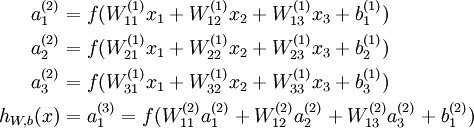
  to denote the i-th input. Given a fixed setting of the parameters W,b, our neural network defines a hypothesis hW,b(x) that outputs a real number. Specifically, the computation that this neural network represents is given by:
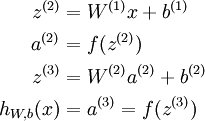
In the sequel, we also let  denote the total weighted sum of inputs to unit i in layer l, including the bias term (e.g.,
 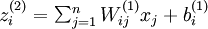 ), so that
  .
.
Note that this easily lends itself to a more compact notation. Specifically, if we extend the activation function to apply to vectors in an element-wise fashion (i.e., f([z1,z2,z3]) = [f(z1),f(z2),f(z3)]), then we can write the equations above more compactly as:
We call this step forward propagation. More generally, recalling that we also use a(1) = x to also denote the values from the input layer, then given layer l‘s activations a(l), we can compute layer l + 1‘s activations a(l + 1) as:
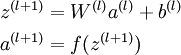
By organizing our parameters in matrices and using matrix-vector operations, we can take advantage of fast linear algebra routines to quickly perform calculations in our network.
We have so far focused on one example neural network, but one can also build neural networks with other architectures (meaning patterns of connectivity between neurons), including ones with multiple hidden layers. The most common choice is a  -layered network where layer
  is the input layer, layer is the output layer, and each layer
  is densely connected to layer
  . In this setting, to compute the output of the network, we can successively compute all the activations in layer
  , then layer
  , and so on, up to layer
  , using the equations above that describe the forward propagation step. This is one example of a feedforward neural network, since the connectivity graph does not have any directed loops or cycles.
Neural networks can also have multiple output units. For example, here is a network with two hidden layers layers L2 and L3 and two output units in layer L4:

To train this network, we would need training examples (x(i),y(i)) where  . This sort of network is useful if there‘re multiple outputs that you‘re interested in predicting. (For example, in a medical diagnosis application, the vector x might give the input features of a patient, and the different outputs yi‘s might indicate presence or absence of different diseases.)
Neural Networks | Backpropagation Algorithm | Gradient checking and advanced optimization | Autoencoders and Sparsity | Visualizing a Trained Autoencoder | Sparse Autoencoder Notation Summary | Exercise:Sparse Autoencoder
Suppose we have a fixed training set  of m training examples. We can train our neural network using batch gradient descent. In detail, for a single training example (x,y), we define the cost function with respect to that single example to be:
This is a (one-half) squared-error cost function. Given a training set of m examples, we then define the overall cost function to be:
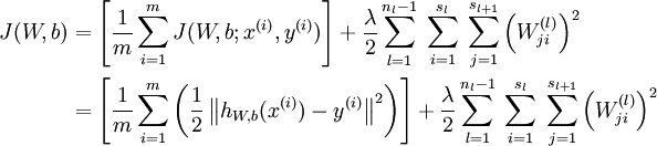
The first term in the definition of J(W,b) is an average sum-of-squares error term. The second term is a regularization term (also called a weight decay term) that tends to decrease the magnitude of the weights, and helps prevent overfitting.
[Note: Usually weight decay is not applied to the bias terms , as reflected in our definition for J(W,b). Applying weight decay to the bias units usually makes only a small difference to the final network, however. If you‘ve taken CS229 (Machine Learning) at Stanford or watched the course‘s videos on YouTube, you may also recognize this weight decay as essentially a variant of the Bayesian regularization method you saw there, where we placed a Gaussian prior on the parameters and did MAP (instead of maximum likelihood) estimation.]
The weight decay parameter λ controls the relative importance of the two terms. Note also the slightly overloaded notation: J(W,b;x,y) is the squared error cost with respect to a single example; J(W,b) is the overall cost function, which includes the weight decay term.
This cost function above is often used both for classification and for regression problems. For classification, we let y = 0 or 1 represent the two class labels (recall that the sigmoid activation function outputs values in [0,1]; if we were using a tanh activation function, we would instead use -1 and +1 to denote the labels). For regression problems, we first scale our outputs to ensure that they lie in the [0,1] range (or if we were using a tanh activation function, then the [ − 1,1] range).
Our goal is to minimize J(W,b) as a function of W and b. To train our neural network, we will initialize each parameter and each to a small random value near zero (say according to a Normal(0,ε2) distribution for some small ε, say 0.01), and then apply an optimization algorithm such as batch gradient descent. Since J(W,b) is a non-convex function, gradient descent is susceptible to local optima; however, in practice gradient descent usually works fairly well. Finally, note that it is important to initialize the parameters randomly, rather than to all 0‘s. If all the parameters start off at identical values, then all the hidden layer units will end up learning the same function of the input (more formally,  will be the same for all values of i, so that
  for any input x). The random initialization serves the purpose of symmetry breaking.
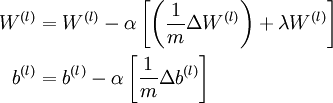
One iteration of gradient descent updates the parameters W,b as follows:
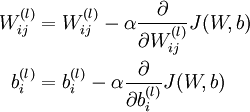
where α is the learning rate. The key step is computing the partial derivatives above. We will now describe the backpropagation algorithm, which gives an efficient way to compute these partial derivatives.
We will first describe how backpropagation can be used to compute 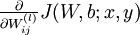 and
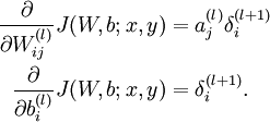
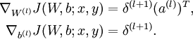
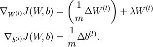
and 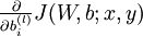 , the partial derivatives of the cost function J(W,b;x,y) defined with respect to a single example (x,y). Once we can compute these, we see that the derivative of the overall cost function J(W,b) can be computed as:
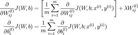
The two lines above differ slightly because weight decay is applied to W but not b.
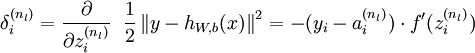
The intuition behind the backpropagation algorithm is as follows. Given a training example (x,y), we will first run a "forward pass" to compute all the activations throughout the network, including the output value of the hypothesis hW,b(x). Then, for each node i in layer l, we would like to compute an "error term"  that measures how much that node was "responsible" for any errors in our output. For an output node, we can directly measure the difference between the network‘s activation and the true target value, and use that to define
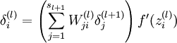
  (where layer nl is the output layer). How about hidden units? For those, we will compute based on a weighted average of the error terms of the nodes that uses as an input. In detail, here is the backpropagation algorithm:
. 

Finally, we can also re-write the algorithm using matrix-vectorial notation. We will use " " to denote the element-wise product operator (denoted ".*" in Matlab or Octave, and also called the Hadamard product), so that if
  , then
  . Similar to how we extended the definition of
  to apply element-wise to vectors, we also do the same for
  (so that
  ).
).
The algorithm can then be written:
, , up to the output layer , using the equations defining the forward propagation steps), set 

Implementation note: In steps 2 and 3 above, we need to compute  for each value of
  . Assuming
  is the sigmoid activation function, we would already have
  stored away from the forward pass through the network. Thus, using the expression that we worked out earlier for
  , we can compute this as
 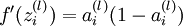 .
.
Finally, we are ready to describe the full gradient descent algorithm. In the pseudo-code below,  is a matrix (of the same dimension as
  ), and
  is a vector (of the same dimension as
  ). Note that in this notation, "" is a matrix, and in particular it isn‘t "
 times ." We implement one iteration of batch gradient descent as follows:
 ,
,  (matrix/vector of zeros) for all .
 to
to  ,
,  and
and  .
. .
.  .
. 
To train our neural network, we can now repeatedly take steps of gradient descent to reduce our cost function  .
.
Backpropagation is a notoriously difficult algorithm to debug and get right, especially since many subtly buggy implementations of it—for example, one that has an off-by-one error in the indices and that thus only trains some of the layers of weights, or an implementation that omits the bias term—will manage to learn something that can look surprisingly reasonable (while performing less well than a correct implementation). Thus, even with a buggy implementation, it may not at all be apparent that anything is amiss. In this section, we describe a method for numerically checking the derivatives computed by your code to make sure that your implementation is correct. Carrying out the derivative checking procedure described here will significantly increase your confidence in the correctness of your code.
Suppose we want to minimize  as a function of
  . For this example, suppose
  , so that
  . In this 1-dimensional case, one iteration of gradient descent is given by
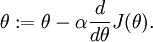
Suppose also that we have implemented some function  that purportedly computes
  , so that we implement gradient descent using the update
 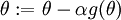 . How can we check if our implementation of
  is correct?
Recall the mathematical definition of the derivative as
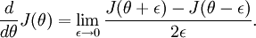
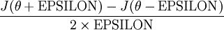
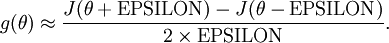
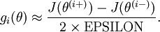
Thus, at any specific value of , we can numerically approximate the derivative as follows:
In practice, we set EPSILON to a small constant, say around  . (There‘s a large range of values of EPSILON that should work well, but we don‘t set EPSILON to be "extremely" small, say
  , as that would lead to numerical roundoff errors.)
Thus, given a function that is supposedly computing , we can now numerically verify its correctness by checking that
The degree to which these two values should approximate each other will depend on the details of  . But assuming
  , you‘ll usually find that the left- and right-hand sides of the above will agree to at least 4 significant digits (and often many more).
Now, consider the case where  is a vector rather than a single real number (so that we have
  parameters that we want to learn), and
  . In our neural network example we used "," but one can imagine "unrolling" the parameters
  into a long vector . We now generalize our derivative checking procedure to the case where may be a vector.
Suppose we have a function  that purportedly computes
  ; we‘d like to check if
  is outputting correct derivative values. Let
  , where
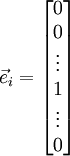
is the -th basis vector (a vector of the same dimension as , with a "1" in the -th position and "0"s everywhere else). So,  is the same as , except its -th element has been incremented by EPSILON. Similarly, let
  be the corresponding vector with the -th element decreased by EPSILON. We can now numerically verify ‘s correctness by checking, for each , that:
When implementing backpropagation to train a neural network, in a correct implementation we will have that
This result shows that the final block of psuedo-code in Backpropagation Algorithm is indeed implementing gradient descent. To make sure your implementation of gradient descent is correct, it is usually very helpful to use the method described above to numerically compute the derivatives of , and thereby verify that your computations of 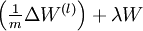 and
and  are indeed giving the derivatives you want.
Finally, so far our discussion has centered on using gradient descent to minimize . If you have implemented a function that computes and  , it turns out there are more sophisticated algorithms than gradient descent for trying to minimize . For example, one can envision an algorithm that uses gradient descent, but automatically tunes the learning rate
  so as to try to use a step-size that causes to approach a local optimum as quickly as possible. There are other algorithms that are even more sophisticated than this; for example, there are algorithms that try to find an approximation to the Hessian matrix, so that it can take more rapid steps towards a local optimum (similar to Newton‘s method). A full discussion of these algorithms is beyond the scope of these notes, but one example is the L-BFGS algorithm. (Another example is the conjugate gradient algorithm.) You will use one of these algorithms in the programming exercise. The main thing you need to provide to these advanced optimization algorithms is that for any , you have to be able to compute and . These optimization algorithms will then do their own internal tuning of the learning rate/step-size (and compute its own approximation to the Hessian, etc.) to automatically search for a value of that minimizes . Algorithms such as L-BFGS and conjugate gradient can often be much faster than gradient descent.
Neural Networks | Backpropagation Algorithm | Gradient checking and advanced optimization | Autoencoders and Sparsity | Visualizing a Trained Autoencoder | Sparse Autoencoder Notation Summary | Exercise:Sparse Autoencoder
So far, we have described the application of neural networks to supervised learning, in which we have labeled training examples. Now suppose we have only a set of unlabeled training examples  , where
  . An autoencoder neural network is an unsupervised learning algorithm that applies backpropagation, setting the target values to be equal to the inputs. I.e., it uses
  .
.
Here is an autoencoder:

The autoencoder tries to learn a function  . In other words, it is trying to learn an approximation to the identity function, so as to output
  that is similar to
  . The identity function seems a particularly trivial function to be trying to learn; but by placing constraints on the network, such as by limiting the number of hidden units, we can discover interesting structure about the data. As a concrete example, suppose the inputs are the pixel intensity values from a
  image (100 pixels) so
  , and there are
  hidden units in layer . Note that we also have
  . Since there are only 50 hidden units, the network is forced to learn a compressed representation of the input. I.e., given only the vector of hidden unit activations
  , it must try to reconstruct the 100-pixel input . If the input were completely random---say, each
  comes from an IID Gaussian independent of the other features---then this compression task would be very difficult. But if there is structure in the data, for example, if some of the input features are correlated, then this algorithm will be able to discover some of those correlations. In fact, this simple autoencoder often ends up learning a low-dimensional representation very similar to PCAs.
Our argument above relied on the number of hidden units  being small. But even when the number of hidden units is large (perhaps even greater than the number of input pixels), we can still discover interesting structure, by imposing other constraints on the network. In particular, if we impose a sparsity constraint on the hidden units, then the autoencoder will still discover interesting structure in the data, even if the number of hidden units is large.
Informally, we will think of a neuron as being "active" (or as "firing") if its output value is close to 1, or as being "inactive" if its output value is close to 0. We would like to constrain the neurons to be inactive most of the time. This discussion assumes a sigmoid activation function. If you are using a tanh activation function, then we think of a neuron as being inactive when it outputs values close to -1.
Recall that  denotes the activation of hidden unit
  in the autoencoder. However, this notation doesn‘t make explicit what was the input that led to that activation. Thus, we will write
  to denote the activation of this hidden unit when the network is given a specific input . Further, let
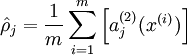
be the average activation of hidden unit (averaged over the training set). We would like to (approximately) enforce the constraint

where  is a sparsity parameter, typically a small value close to zero (say
  ). In other words, we would like the average activation of each hidden neuron to be close to 0.05 (say). To satisfy this constraint, the hidden unit‘s activations must mostly be near 0.
To achieve this, we will add an extra penalty term to our optimization objective that penalizes  deviating significantly from . Many choices of the penalty term will give reasonable results. We will choose the following:
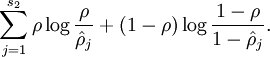
Here, is the number of neurons in the hidden layer, and the index is summing over the hidden units in our network. If you are familiar with the concept of KL divergence, this penalty term is based on it, and can also be written
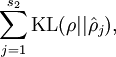
where  is the Kullback-Leibler (KL) divergence between a Bernoulli random variable with mean and a Bernoulli random variable with mean . KL-divergence is a standard function for measuring how different two different distributions are. (If you‘ve not seen KL-divergence before, don‘t worry about it; everything you need to know about it is contained in these notes.)
This penalty function has the property that  if
if  , and otherwise it increases monotonically as diverges from . For example, in the figure below, we have set
  , and plotted
  for a range of values of :

We see that the KL-divergence reaches its minimum of 0 at , and blows up (it actually approaches  ) as approaches 0 or 1. Thus, minimizing this penalty term has the effect of causing to be close to .
Our overall cost function is now
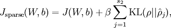
where is as defined previously, and  controls the weight of the sparsity penalty term. The term (implicitly) depends on also, because it is the average activation of hidden unit , and the activation of a hidden unit depends on the parameters .
To incorporate the KL-divergence term into your derivative calculation, there is a simple-to-implement trick involving only a small change to your code. Specifically, where previously for the second layer ( ), during backpropagation you would have computed
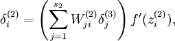
now instead compute
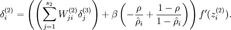
One subtlety is that you‘ll need to know  to compute this term. Thus, you‘ll need to compute a forward pass on all the training examples first to compute the average activations on the training set, before computing backpropagation on any example. If your training set is small enough to fit comfortably in computer memory (this will be the case for the programming assignment), you can compute forward passes on all your examples and keep the resulting activations in memory and compute the s. Then you can use your precomputed activations to perform backpropagation on all your examples. If your data is too large to fit in memory, you may have to scan through your examples computing a forward pass on each to accumulate (sum up) the activations and compute (discarding the result of each forward pass after you have taken its activations
  into account for computing ). Then after having computed , you‘d have to redo the forward pass for each example so that you can do backpropagation on that example. In this latter case, you would end up computing a forward pass twice on each example in your training set, making it computationally less efficient.
The full derivation showing that the algorithm above results in gradient descent is beyond the scope of these notes. But if you implement the autoencoder using backpropagation modified this way, you will be performing gradient descent exactly on the objective  . Using the derivative checking method, you will be able to verify this for yourself as well.
Neural Networks | Backpropagation Algorithm | Gradient checking and advanced optimization | Autoencoders and Sparsity | Visualizing a Trained Autoencoder | Sparse Autoencoder Notation Summary | Exercise:Sparse Autoencoder
Having trained a (sparse) autoencoder, we would now like to visualize the function learned by the algorithm, to try to understand what it has learned. Consider the case of training an autoencoder on images, so that . Each hidden unit computes a function of the input:
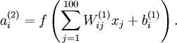
We will visualize the function computed by hidden unit ---which depends on the parameters  (ignoring the bias term for now)---using a 2D image. In particular, we think of as some non-linear feature of the input . We ask: What input image would cause to be maximally activated? (Less formally, what is the feature that hidden unit is looking for?) For this question to have a non-trivial answer, we must impose some constraints on . If we suppose that the input is norm constrained by
  , then one can show (try doing this yourself) that the input which maximally activates hidden unit is given by setting pixel
  (for all 100 pixels,
  ) to
) to
By displaying the image formed by these pixel intensity values, we can begin to understand what feature hidden unit is looking for.
If we have an autoencoder with 100 hidden units (say), then we our visualization will have 100 such images---one per hidden unit. By examining these 100 images, we can try to understand what the ensemble of hidden units is learning.
When we do this for a sparse autoencoder (trained with 100 hidden units on 10x10 pixel inputs1 we get the following result:

Each square in the figure above shows the (norm bounded) input image that maximally actives one of 100 hidden units. We see that the different hidden units have learned to detect edges at different positions and orientations in the image.
These features are, not surprisingly, useful for such tasks as object recognition and other vision tasks. When applied to other input domains (such as audio), this algorithm also learns useful representations/features for those domains too.
1 The learned features were obtained by training on whitened natural images. Whitening is a preprocessing step which removes redundancy in the input, by causing adjacent pixels to become less correlated.
Neural Networks | Backpropagation Algorithm | Gradient checking and advanced optimization | Autoencoders and Sparsity | Visualizing a Trained Autoencoder | Sparse Autoencoder Notation Summary | Exercise:Sparse Autoencoder
Here is a summary of the symbols used in our derivation of the sparse autoencoder:
| Symbol | Meaning |
|---|---|
|
Input features for a training example,  . . |
 |
Output/target values. Here, can be vector valued. In the case of an autoencoder,  . . |
 |
The -th training example |
 |
Output of our hypothesis on input , using parameters . This should be a vector of
the same dimension as the target value |
 |
The parameter associated with the connection between unit in layer , and
unit |
 |
The bias term associated with unit in layer . Can also be thought of as the parameter associated with the connection between the bias unit in layer and unit in layer . |
|
Our parameter vector. It is useful to think of this as the result of taking the parameters and ``unrolling them into a long column vector. |
|
Activation (output) of unit in layer of the network.
In addition, since layer |
|
The activation function. Throughout these notes, we used  . . |
 |
Total weighted sum of inputs to unit in layer . Thus,  . . |
|
Learning rate parameter |
 |
Number of units in layer (not counting the bias unit). |
|
Number layers in the network. Layer  is usually the input layer, and layer the output layer. is usually the input layer, and layer the output layer. |
 |
Weight decay parameter. |
|
For an autoencoder, its output; i.e., its reconstruction of the input . Same meaning as . |
|
Sparsity parameter, which specifies our desired level of sparsity |
|
The average activation of hidden unit (in the sparse autoencoder). |
|
Weight of the sparsity penalty term (in the sparse autoencoder objective). |
Neural Networks | Backpropagation Algorithm | Gradient checking and advanced optimization | Autoencoders and Sparsity | Visualizing a Trained Autoencoder | Sparse Autoencoder Notation Summary | Exercise:Sparse Autoencoder
Contents[hide] |
In this problem set, you will implement the sparse autoencoder algorithm, and show how it discovers that edges are a good representation for natural images. (Images provided by Bruno Olshausen.) The sparse autoencoder algorithm is described in the lecture notes found on the course website.
In the file sparseae_exercise.zip, we have provided some starter code in Matlab. You should write your code at the places indicated in the files ("YOUR CODE HERE"). You have to complete the following files: sampleIMAGES.m, sparseAutoencoderCost.m, computeNumericalGradient.m. The starter code in train.m shows how these functions are used.
Specifically, in this exercise you will implement a sparse autoencoder, trained with 8×8 image patches using the L-BFGS optimization algorithm.
A note on the software: The provided .zip file includes a subdirectory minFunc with 3rd party software implementing L-BFGS, that is licensed under a Creative Commons, Attribute, Non-Commercial license. If you need to use this software for commercial purposes, you can download and use a different function (fminlbfgs) that can serve the same purpose, but runs ~3x slower for this exercise (and thus is less recommended). You can read more about this in the Fminlbfgs_Details page.
The first step is to generate a training set. To get a single training example x, randomly pick one of the 10 images, then randomly sample an 8×8 image patch from the selected image, and convert the image patch (either in row-major order or column-major order; it doesn‘t matter) into a 64-dimensional vector to get a training example 
Complete the code in sampleIMAGES.m. Your code should sample 10000 image patches and concatenate them into a 64×10000 matrix.
To make sure your implementation is working, run the code in "Step 1" of train.m. This should result in a plot of a random sample of 200 patches from the dataset.
Implementational tip: When we run our implemented sampleImages(), it takes under 5 seconds. If your implementation takes over 30 seconds, it may be because you are accidentally making a copy of an entire 512×512 image each time you‘re picking a random image. By copying a 512×512 image 10000 times, this can make your implementation much less efficient. While this doesn‘t slow down your code significantly for this exercise (because we have only 10000 examples), when we scale to much larger problems later this quarter with 106 or more examples, this will significantly slow down your code. Please implement sampleIMAGES so that you aren‘t making a copy of an entire 512×512 image each time you need to cut out an 8x8 image patch.
Implement code to compute the sparse autoencoder cost function Jsparse(W,b) (Section 3 of the lecture notes) and the corresponding derivatives of Jsparse with respect to the different parameters. Use the sigmoid function for the activation function,  . In particular, complete the code in sparseAutoencoderCost.m.
The sparse autoencoder is parameterized by matrices  ,
,  vectors
  ,
,  . However, for subsequent notational convenience, we will "unroll" all of these parameters into a very long parameter vector θ with s1s2 + s2s3 + s2 + s3 elements. The code for converting between the (W(1),W(2),b(1),b(2)) and the θ parameterization is already provided in the starter code.
Implementational tip: The objective Jsparse(W,b) contains 3 terms, corresponding to the squared error term, the weight decay term, and the sparsity penalty. You‘re welcome to implement this however you want, but for ease of debugging, you might implement the cost function and derivative computation (backpropagation) only for the squared error term first (this corresponds to setting λ = β = 0), and implement the gradient checking method in the next section to first verify that this code is correct. Then only after you have verified that the objective and derivative calculations corresponding to the squared error term are working, add in code to compute the weight decay and sparsity penalty terms and their corresponding derivatives.
Following Section 2.3 of the lecture notes, implement code for gradient checking. Specifically, complete the code in computeNumericalGradient.m. Please use EPSILON = 10-4 as described in the lecture notes.
We‘ve also provided code in checkNumericalGradient.m for you to test your code. This code defines a simple quadratic function  given by
  , and evaluates it at the point x = (4,10)T. It allows you to verify that your numerically evaluated gradient is very close to the true (analytically computed) gradient.
After using checkNumericalGradient.m to make sure your implementation is correct, next use computeNumericalGradient.m to make sure that your sparseAutoencoderCost.m is computing derivatives correctly. For details, see Steps 3 in train.m. We strongly encourage you not to proceed to the next step until you‘ve verified that your derivative computations are correct.
Implementational tip: If you are debugging your code, performing gradient checking on smaller models and smaller training sets (e.g., using only 10 training examples and 1-2 hidden units) may speed things up.
Now that you have code that computes Jsparse and its derivatives, we‘re ready to minimize Jsparse with respect to its parameters, and thereby train our sparse autoencoder.
We will use the L-BFGS algorithm. This is provided to you in a function called minFunc (code provided by Mark Schmidt) included in the starter code. (For the purpose of this assignment, you only need to call minFunc with the default parameters. You do not need to know how L-BFGS works.) We have already provided code in train.m (Step 4) to call minFunc. The minFunc code assumes that the parameters to be optimized are a long parameter vector; so we will use the "θ" parameterization rather than the "(W(1),W(2),b(1),b(2))" parameterization when passing our parameters to it.
Train a sparse autoencoder with 64 input units, 25 hidden units, and 64 output units. In our starter code, we have provided a function for initializing the parameters. We initialize the biases to zero, and the weights to random numbers drawn uniformly from the interval  , where nin is the fan-in (the number of inputs feeding into a node) and nout is the fan-in (the number of units that a node feeds into).
The values we provided for the various parameters (λ,β,ρ, etc.) should work, but feel free to play with different settings of the parameters as well.
Implementational tip: Once you have your backpropagation implementation correctly computing the derivatives (as verified using gradient checking in Step 3), when you are now using it with L-BFGS to optimize Jsparse(W,b), make sure you‘re not doing gradient-checking on every step. Backpropagation can be used to compute the derivatives of Jsparse(W,b) fairly efficiently, and if you were additionally computing the gradient numerically on every step, this would slow down your program significantly.
After training the autoencoder, use display_network.m to visualize the learned weights. (See train.m, Step 5.) Run "print -djpeg weights.jpg" to save the visualization to a file "weights.jpg" (which you will submit together with your code).
To successfully complete this assignment, you should demonstrate your sparse autoencoder algorithm learning a set of edge detectors. For example, this was the visualization we obtained:

Our implementation took around 5 minutes to run on a fast computer. In case you end up needing to try out multiple implementations or different parameter values, be sure to budget enough time for debugging and to run the experiments you‘ll need.
Also, by way of comparison, here are some visualizations from implementations that we do not consider successful (either a buggy implementation, or where the parameters were poorly tuned):


Neural Networks | Backpropagation Algorithm | Gradient checking and advanced optimization | Autoencoders and Sparsity | Visualizing a Trained Autoencoder | Sparse Autoencoder Notation Summary | Exercise:Sparse Autoencoder
【转帖】Andrew ng 【Sparse Autoencoder 】@UFLDL Tutorial
标签:des style blog http ar io os sp for
原文地址:http://www.cnblogs.com/daleloogn/p/4170451.html
 .
.