加州大学伯克利分校Stat2.3x Inference 统计推断学习笔记: Section 5 Window to a Wider World

标签：

Stat2.3x Inference（统计推断）课程由加州大学伯克利分校（University of California, Berkeley）于2014年在edX平台讲授。

PDF笔记下载（Academia.edu）

Summary

Chi-square test

• Random sample or not / Good or bad
  • $$H_0: \text{Good model}$$ $$H_A: \text{Not good model}$$
  • Based on the expected proportion to calculate the expected values
  • $\chi^2$ statistic is $$\chi^2=\sum{\frac{(o-e)^2}{e}}$$ where $o$ is observed values, $e$ is expected values.
  • The degree of freedom is the number of categories minus one
  • Follows approximately the $\chi^2$ distribution, we can calculate its P-value by using R function:

    1-pchisq(chi, df)

• Independent or not
  • $$H_0: \text{Independent}$$ $$H_A: \text{not Independent}$$
  • Contingency table
  • Under $H_0$, in each cell of the table $$\text{expected count}=\frac{\text{row total}\times\text{column total}}{\text{grand total}}$$ That is, $P(A\cap B)=P(A)\cdot P(B)$ under the independent assumption.
  • $\chi^2$ statistic is $$\chi^2=\sum{\frac{(o-e)^2}{e}}$$ where $o$ is observed values, $e$ is expected values.
  • The degree of freedom is $(\text{row}-1)\times(\text{column}-1)$
  • Follows approximately the $\chi^2$ distribution, we can calculate its P-value by using R function:

    1-pchisq(chi, df)

ADDITIONAL PRACTICE PROBLEMS FOR WEEK 5

The population is all patients at a large system of hospitals; each sampled patient was classified by the type of room he/she was in, and his/her level of satisfaction with the care received. The question is whether type of room is independent of level of satisfaction.

1. What are the null and alternative hypotheses?

2. Under the null, what is the estimated expected number of patients in the "shared room, somewhat satisfied" cell?

3. Degrees of freedom = ( )

4. The chi-square statistic is about 13.8. Roughly what is the P-value, and what is the conclusion of the test?

Solution

1. Null: The two variables are independent; Alternative: The two variables are not independent.

2. We need to expand the original table:

Thus the estimated expected number of patients in the shared room, somewhat satisfied is $$784\times\frac{322}{784}\times\frac{255}{784}=104.7321$$

3. Degree of freedom is $(3-1)\times(3-1)=4$

4. P-value is 0.007961505 which is smaller than 0.05, so we reject $H_0$. That is, the conclusion is the two variables are not independent. R code:

1 - pchisq(13.8, 4)
[1] 0.007961505

UNGRADED EXERCISE SET A PROBLEM 1

According to a genetics model, plants of a particular species occur in the categories A, B, C, and D, in the ratio 9:3:3:1. The categories of different plants are mutually independent. At a lab that grows these plants, 218 are in Category A, 69 in Category B, 84 in Category C, and 29 in Category D. Does the model look good? Follow the steps in Problems 1A-1F.

1A The null hypothesis is:

a. The model is good.

b. The model isn‘t good.

c. Too many of the plants are in Category C.

d. The proportion of plants in Category A is expected to be 9/16; the difference in the sample is due to chance.

1B The alternative hypothesis is:

a. The model is good.

b. The model isn‘t good.

c. Too many of the plants are in Category C.

d. The proportion of plants in Category A is expected to be 9/16; the difference in the sample is due to chance.

1C Under the null, the expected number of plants in Category D is( ).

1D The chi-square statistic is closest to

a. 1 b. 1.5 c. 2 d. 2.5 e. 3 f. 3.5 g. 4 h. 4.5

1E Degrees of freedom = ( ).

1F Based on this test, does the model look good? Yes No

Solution

1A) The null hypothesis is "the model is good". (a) is correct.

1B) The alternative hypothesis is "the model is not good". (b) is correct.

1C) The expected number of plants in Category D is $$(218+69+84+29)\times\frac{1}{9+3+3+1}=25$$

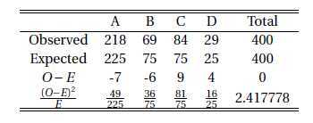
1D) (d) is correct. We can use the following table

R code:

o = c(218, 69, 84, 29)
e = c(225, 75, 75, 25)
chi = sum((o - e)^2 / e); chi
[1] 2.417778

1E) Degree of freedom is $4-1=3$.

1F) P-value is 0.4903339 which is larger than 0.05, so we reject $H_A$. The conclusion is "the model is good". R code:

1 - pchisq(chi, 3)
[1] 0.4903339

PROBLEM 2

A simple random sample of cars in a city was categorized according to fuel type and place of manufacture.

Are place of manufacture and fuel type independent? Follow the steps in Problems 2A-2D.

2A If the two variables were independent, the chance that a sampled car is a domestic gasoline fueled car would be estimated to be about

0.0362 0.0499 0.2775 0.3820 0.5

2B If the two variables were independent, the expected number of foreign gas/electric hybrids would be estimated to be ( ). (Please keep at least two decimal places; by now you should understand why you should not round off to an integer.)

2C Degrees of freedom =( )

1 2 3 4

2D The chi-square statistic is 0.6716. The test therefore concludes that the two variables are independent not independent

Solution

2A) Expand the table:

If the two variables were independent, then $$P(\text{domestic gasoline})=P(\text{domestic})\cdot P(\text{gasoline})=\frac{215}{511}\times\frac{337}{511}=0.2774767\doteq 0.2775$$

2B) If the two variables were independent, then $$511\times P(\text{foreign gasoline/electricity})=511\times\frac{296}{511}\times\frac{130}{511}=75.30333$$

2C) Degree of freedom is $(2-1)\times(3-1)=2$.

2D) The P-value is 0.714766 which is larger than 0.05, so we reject $H_A$. That is, the conclusion is independent. R code:

1 - pchisq(0.6716, 2)
[1] 0.714766

We can calculate $\chi^2$ statistic by using R built-in function

chisq.test()

data = matrix(c(146, 18, 51, 191, 26, 79), ncol = 2)
  chisq.test(data)

 Pearson‘s Chi-squared test

data:  data
X-squared = 0.6716, df = 2, p-value = 0.7148

加州大学伯克利分校Stat2.3x Inference 统计推断学习笔记: Section 5 Window to a Wider World

标签：

原文地址：http://www.cnblogs.com/zhaoyin/p/4179331.html