标签:
本书中的例子包括在nutshell的R包中,使用数据,需加载nutshell包
install.packages("nutshell")
R provides a way to run a large set of commands in sequence and save the results to a file.
以batch mode运行R的一种方式是:使用系统命令行(不是R控制台)。,通过命令行运行R的好处是不用启动R就可以运行一系列命令。这对于自动化分析非常有帮助。,
更多关于从命令行运行R的信息运行以下命令查看
$ R CMD BATCH+R脚本
$ R --help
# 批运行R脚本的第二个命令
$ RScript+R脚本
# 在R内批运行R脚本,使用:
Source命令
RExcel软件(http://rcom.univie.ac.at / http://rcom.univie.ac.at/download.html)
如果已经安装了R,直接可以安装RExcel包,下面的代码执行以下路径:
Download RExcelàconfigure the RCOM服务器—>安装RDCOMà启动RExcel安装器
> install.packages("RExcelInstaller", "rcom", "rsproxy") # 这种安装方式不行 > # configure rcom > library(rcom) > comRegisterRegistry() > library(RExcelInstaller) > # execute the following command in R to start the installer for RDCOM > installstatconnDCOM() > # execute the following command in R to start the installer for REXCEL > installRExcel() |
安装了RExcel之后,就可以在Excel的菜单项中访问RExcel啦!!!
As a web application
The rApache software allows you to incorporate analyses from R into a web
application. (For example, you might want to build a server that shows sophisticated
reports using R lattice graphics.) For information about this project, see
http://biostat.mc.vanderbilt.edu/rapache/.
As a server
The Rserve software allows you to access R from within other applications. For
example, you can produce a Java program that uses R to perform some calculations.
As the name implies, Rserver is implemented as a network server, so a
single Rserve instance can handle calculations from multiple users on different
machines. One way to use Rserve is to install it on a heavy-duty server with lots
of CPU power and memory, so that users can perform calculations that they
couldn‘t easily perform on their own desktops. For more about this project, see
http://www.rforge.net/Rserve/index.html.
As we described above, you can also use R Studio to run R on a server and access
if from a web browser.
Inside Emacs
The ESS (Emacs Speaks Statistics) package is an add-on for Emacs that allows
you to run R directly within Emacs. For more on this project, see http://ess.r-project.org/
向量是最简单的数据结构,数组是一个多维向量,矩阵是一个二维数据;
数据框一个列表(包含了多个长度相同的命名向量!),很像一个电子表格或数据库表。
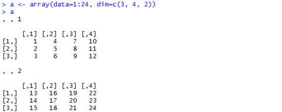
@定义一个数组
> a <- array(c(1, 2, 3, 4, 5, 6, 7, 8, 9, 10, 11, 12), dim=c(3, 4))
Here is what the array looks like:
> a
[,1] [,2] [,3] [,4]
[1,] 1 4 7 10
[2,] 2 5 8 11
[3,] 3 6 9 12
And here is how you reference one cell:
> a[2,2]
[1] 5
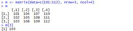
@定义一个矩阵
> m <- matrix(data=c(1,2,3,4,5,6,7,8,9,10,11,12),nrow=3,ncol=4)
> m
[,1] [,2] [,3] [,4]
[1,] 1 4 7 10
[2,] 2 5 8 11
[3,] 3 6 9 12
@定义一个数据框
> teams <- c("PHI","NYM","FLA","ATL","WSN")
> w <- c(92, 89, 94, 72, 59)
> l <- c(70, 73, 77, 90, 102)
> nleast <- data.frame(teams,w,l)
> nleast
teams w l
1 PHI 92 70
2 NYM 89 73
3 FLA 94 77
4 ATL 72 90
5 WSN 59 102
R中的每一个对象都有一个类型。此外,每一个对象都是一个类的成员。
可以使用class函数来确定一个对象的类,例如:
> class(class)
[1] "function"
> class(mtcars)
[1] "data.frame"
> class(letters)
[1] "character"
不同类的方法可以有相同的名称,这些方法被称为泛函数(generic function)。
比如,+是一个adding objects的泛函。它可以执行数值相加,日期相加等,如下
> 17 + 6
[1] 23
> as.Date("2009-09-08") + 7
[1] "2009-09-15"
顺便提一下,R解释器会调用print(x)函数来打印结果,这意味着,如果我们定义了一个新的类,可以定义一个print方法来指定从该新类中生成的对象如何显示在控制台上!
To statisticians, a model is a concise way to describe a set of data, usually with a mathematical formula. Sometimes, the goal is to build a predictive model with training data to predict values based on other data. Other times, the goal is to build a descriptive model that helps you understand the data better.
R has a special notation for describing relationships between variables. Suppose that
you are assuming a linear model for a variable y, predicted from the variables x1,
x2, ..., xn. (Statisticians usually refer to y as the dependent variable, and x1, x2, ...,
xn as the independent variables.)。在方程中,可以表示为

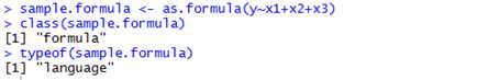
在R中,将这种关系写成 ,这是公式对象的一种形式。
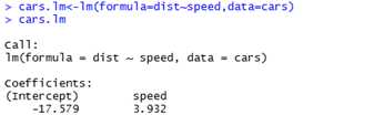
以base包中的car数据集为例,简单解释一下公式对象的用法。Car数据集显示了不同车的speed和stopping distance。我们假设stopping distance是speed的一个线性函数,因此,使用线性回归来估计两者的关系。公式可以写成:dist~speed。使用lm函数来估计模型的参数,该函数返回一个lm类对象。
For some more information,使用summary函数
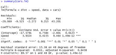
可以看到,summary函数显示了function call,拟合参数的分布(the distribution
of the residuals from the fit),相关系数(coefficients)以及拟合信息。
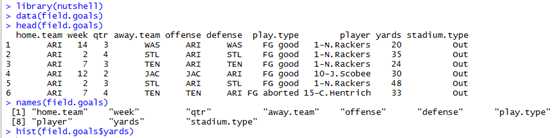
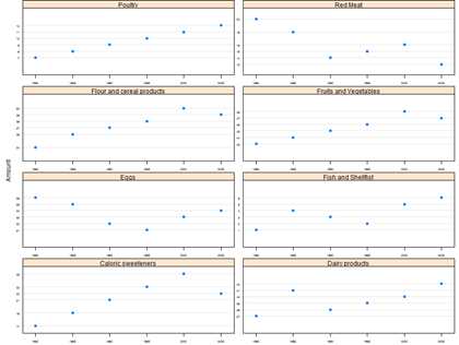
R包括了各种数据可视化包:graphics、grid、lattice。为了简单解释一下图形功能,使用国家足球队的射门得分尝试(field goal attempts)数据(来自nutshell包)来演示。一个队在一组球门中踢球,进球得3分。如果丢掉一个射门球,则将足球交给其他队。
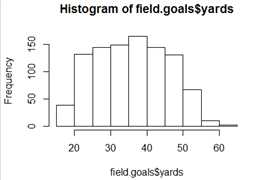
????@首先,来看看距离(distance)的分布。这里使用hist函数
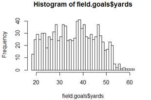
进一步叫做breaks参数来向直方图中添加更多的bins

@ 使用lattice包来一个例子
数据集(we‘ll look at how American eating habits changed between 1980
and 2005:来自nutshell包)。
具体地说,我们要查看how amount(The amount of food consumed) varies by year,同时还要针对Food变量的每一个值分别绘制趋势。在lattice包中,我们通过一个公式来指定想要绘图的数据,在本例中,形如:Amount ~ Year | Food。
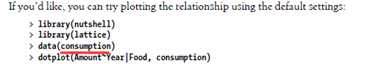
然而,默认图形可读性弱,axis标签(lables)太大,每幅图的scale(纵横比)相同,因此需要做一些微调。
> library(lattice)
> data(consumption)
> dotplot(Amount~Year|Food,consumption,aspect="xy",scales=list(relation=‘sliced‘,cex=.4))
# The aspect option changes the aspect ratios of each plot to try to show changes from
45° angles (making changes easier to see). The scales option changes how the axes
are drawn.
@ 获取关于一个函数的帮助,如glm
# help(glm)------>?glm
@ 对于特殊字符如 +,需要将其放在backquotes(反引号)中
#?‘+‘
@ 查看一个帮助文件中的例子,比如查看glm中的例子
# example(glm)
@ 可以搜索关于一个话题(topic)的吧帮助,比如"回归",使用help.searceh函数
# help.search("regression")
一种简便的方式是直接使用:??regression
@ 获取一个包的帮助文件,比如获取grDevices包的帮助,使用
# library(help=‘grDevices‘)
@ vignette函数
1)一些包(特别是来自Bioconductor)会包含至少一个vignette,一个vignette是关于如何使用包的简短描述(带例子)。例如,查看affy包的vignette(前提是要已安装affy包),使用
# vignette("affy")
2)查看所有附加包(attached packages)的可用vignettes,使用
# vignette(all=FALSE)
3)查看所有已安装包的vignettes,使用
# vignette(all=TRUE)
使用包的第一步:将包安装到本例库中(local library);第二步:将包加载到当前工作区中(current session)。
R的帮助系统会随着越来越多的search包而变得异常慢。two packages may both use
functions with names like "fit" that work very differently, resulting in strange and
unexpected results. By loading only packages that you need, you can minimize the
chance of these conflicts。
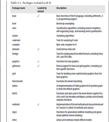
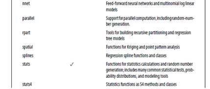
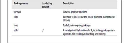
@ To get the list of packages loaded by default,
# getOption("defaultPackages")

This command omits the base package; the base package implements many key
features of the R language and is always loaded.
@ 查看当前已加载包的列表,使用
# (.packages())

@ 查看所有可用包,使用
(.packages(all.available=TRUE))
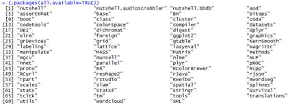
@ 还可以使用不带参数的library( )命令,这会弹出一个新窗口,显示可用包的集合。
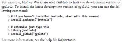
两个最大的包来源是:CRAN (Comprehensive R Archive Network) and Bioconductor,另外一个是R-Forge。还有比如:GitHub。
全部可用包的查询地址
Repository URL
CRAN See http://cran.r-project.org/web/packages/ for an authoritative list, but you should try to find your local
mirror and use that site instead
Bioconductor http://www.bioconductor.org/packages/release/Software.html
R-Forge http://r-forge.r-project.org/
> install.packages(c("tree","maptree")) #安装包到默认位置
> remove.packages(c("tree", "maptree"),.Library) #从库中删除包
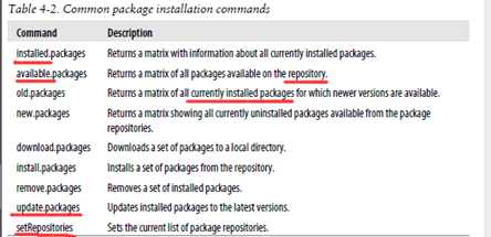
常用的包相关命令
创建一个包目录(package directory)
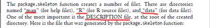
创建包时,需要将所有的包文件(代码、数据、文档等)放在一个单个的目录中。可以使用package.skeleton函数来创建合适的目录结构,如下:
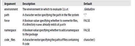
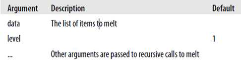
package.skeleton(name = "anRpackage", list, environment = .GlobalEnv, path = ".", force = FALSE, namespace = FALSE, code_files = character())? |
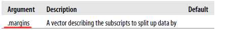
这个函数还可以将R一组R对象复制到该目录下。下面是其参数的一些描述
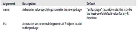
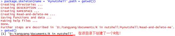

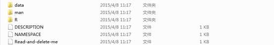
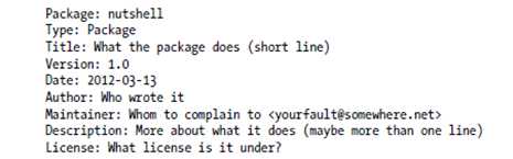
Package.skeleton函数会创建几个文件:名称man的帮助文件目录,R源文件,data数据文件,DESCPRITION文件
R includes a set of functions that help automate the creation of help files for packages:
prompt (for generic documentation), promptData (for documenting data files),
promptMethods (for documenting methods of a generic function), and promptClass
(for documenting a class). See the help files for these functions for additional
information.
You can add data files to the data directory in several different forms: as R data files
(created by the save function and named with either a .rda or a .Rdata suffix), as
comma-separated value files (with a .csv suffix), or as an R source file containing R
code (with a .R suffix).
创建包
????在将所有的资料(materials)添加到包之后。可以通过命令行来建立包,在这之前,请确保,创建的包符合CRAN规则。使用check命令
# $ R CMD check nutshell
# $ R CMD CHECK –help :获取更多CMD check命令的信息
# $ R CMD build nutshell:创建包(build the package)
更多可用的建包参考http://cran.r-project.org/doc/manuals/R-exts.pdf.
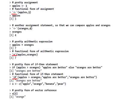
表达式包括assignment statements, conditional statements, and arithmetic expressions
看几个例子:
> x <- 1
> if (1 > 2) "yes" else "no"
[1] "no"
> 127 %% 10
[1] 7
表达式由对象和函数构成,可用通过换行或用分号(semicolons)来分隔表达式,例如
> "this expression will be printed"; 7 + 13; exp(0+1i*pi)
[1] "this expression will be printed"
[1] 20
[1] -1+0i
R中对象的例子包括:numeric,vectors, character vectors, lists, and functions
> # a numerical vector (with five elements)
> c(1,2,3,4,5)
[1] 1 2 3 4 5
> # a character vector (with one element)
> "This is an object too"
[1] "This is an object too"
> # a list
> list(c(1,2,3,4,5),"This is an object too", " this whole thing is a list")
[[1]]
[1] 1 2 3 4 5
[[2]]
[1] "This is an object too"
[[3]]
[1] " this whole thing is a list"
> # a function
> function(x,y) {x + y}
function(x,y) {x + y}
R中的变量名被称为符号。当你对一个变量名赋予一个对象时,实际上是将对象赋给一个当前环境中的符号。例如: x <- 1(assigns the symbol "x" to the object "1" in the current environment)。
A function is an object in R that takes some input objects (called the arguments of
the function) and returns an output object。例如
> animals <- c("cow", "chicken", "pig", "tuba")
> animals[4] <- "duck" #将第四个元素改成duck
上面的语句被解析成对[<-函数的调用,等价于
> `[<-`(animals,4,"duck")

一些其他R语法和响应函数调用的例子
四个特殊值:NA+Inf/-Inf+NaN+NULL
NA用于代表缺失值(not available)。如下:
> v <- c(1,2,3)
> v
[1] 1 2 3
> length(v) <- 4 # 扩展向量/矩阵/数组的大小超过了值定义的范围。新的空间就会用NA来代替.
> v
[1] 1 2 3 NA
Inf和-Inf代表positive and negative infinity
当一个计算结果太大时,R就会返回该值,例如
> 2 ^ 1024
[1] Inf
> - 2 ^ 1024
[1] –Inf
当除以0时也会返回该值
> 1 / 0
[1] Inf
NaN代表无意义的结果(not a number)
当计算的结果无意义时,返回该值,如下(a computation will produce a result that makes little sense)
> Inf - Inf
[1] NaN
> 0 / 0
[1] NaN
NULL经常被用作函数的一个参数,用来代表no value was assigned to the argument。有一些函数也可能返回NULL值。
下面是强转规则的概述
? Logical values are converted to numbers: TRUE is converted to 1 and FALSE to 0.
? Values are converted to the simplest type required to represent all information.
? The ordering is roughly logical < integer < numeric < complex < character < list.
? Objects of type raw are not converted to other types.
? Object attributes are dropped when an object is coerced from one type to
another.
当传递参数给函数时,可以使用AsIs函数(或I函数)来阻止强转。
> if (x > 1) "orange" else "apple"
[1] "apple"
对于上面这句话,为了展示这个表达式如何被解析的,使用quote()函数,该函数会解析参数,调用quote,一个R表达式会返回一个language对象。
> typeof(quote(if (x > 1) "orange" else "apple"))
[1] "language"
> quote(if (x > 1) "orange" else "apple")
if (x > 1) "orange" else "apple"
当从这句话看不出什么思路,可以将一个language对象转化成一个列表,得到上述表达式的解析树(parse tree)
> as(quote(if (x > 1) "orange" else "apple"),"list") # as函数将一个对象转化成一个指定的类
[[1]]
`if`
[[2]]
x > 1
[[3]]
[1] "orange"
[[4]]
[1] "apple"
还可以对列表中的每一个元素运行typeof函数以便查看每个对象的类型
> lapply(as(quote(if (x > 1) "orange" else "apple"), "list"),typeof)
[[1]]
[1] "symbol"
[[2]]
[1] "language"
[[3]]
[1] "character"
[[4]]
[1] "character"
可以看到if-then语句没有被包括在解析表达式中(特别是else关键字)。
逆句法分析(deparse)函数
The deparse function can take the parse tree and turn it back into properly formatted R code(The deparse function will use proper R syntax when translating a language object back into the original code)
> deparse(quote(x[2]))
[1] "x[2]"
> deparse(quote(`[`(x,2)))
[1] "x[2]"
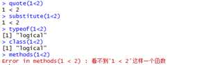
As you read through this book, you might want to try using quote, substitute,typeof, class, and methods to see how the R interpreter parses expressions
Constants are the basic building blocks for data objects in R: numbers, character values, and symbols.
Many functions in R can be written as operators. An operator is a function that takes one or two arguments and can be written without parentheses.
加减乘除+取模等
用户自定二元运算符由一个包括在两个%%字符之间的字符串构成,如下
> `%myop%` <- function(a, b) {2*a + 2*b}
> 1 %myop% 1
[1] 4
> 1 %myop% 2
[1] 6
运算符顺序
? Function calls and grouping expressions
? Index and lookup operators
? Arithmetic
? Comparison
? Formulas
? Assignment
? Help
Table 6-1 shows a complete list of operators in R and their precedence.

大多数赋值都是将一个对象简单地赋给一个符号(即变量),例如
> x <- 1
> y <- list(shoes="loafers", hat="Yankees cap", shirt="white")
> z <- function(a, b, c) {a ^ b / c}
> v <- c(1, 2, 3, 4, 5, 6, 7, 8)
有一种赋值语句,和常见的赋值语句不通。因为带函数的赋值在赋值运算符的左边。例如
> dim(v) <- c(2, 4)
> v[2, 2] <- 10
> formals(z) <- alist(a=1, b=2, c=3)
这背后的逻辑是,形如下面的赋值语句
fun(sym) <- val #一般说来,fun表示由sym代表的对象的一个属性。
R提供了对表达式分组的不通方式:分号,括号,大括号(semicolons,
parentheses, and curly braces)。
@ 分隔表达式(separating expressions)
You can write a series of expressions on separate lines:
> x <- 1
> y <- 2
> z <- 3
Alternatively, you can place them on the same line, separated by semicolons:
> x <- 1; y <- 2; z <- 3
@ 括号(parentheses)
圆括号(parentheses notation)返回括号中表达式计算后的结果,可用于复写运算符默认的顺序!
> 2 * (5 + 1)
[1] 12
> # equivalent expression
> f <- function (x) x
> 2 * f(5 + 1)
[1] 12
@ 大花括号(curly braces)
{expression_1; expression_2; ... expression_n}
通常,用于将一组操作分组在函数体中
> f <- function() {x <- 1; y <- 2; x + y}
> f()
[1] 3
然而,圆括号还可以用于以下情况
> {x <- 1; y <- 2; x + y}
[1] 3
区别在于:
我们已经讨论了两个重要的结构集:operators和groupin brackets。继续深入介绍
?
@ 条件语句(conditional statements)
# 两种形式
if (condition) true_expression else false_expression;或者
if (condition) expression
因为其中的真假表达式不总是被估值,所以if的类型是special
> typeof(`if`)
[1] "special"
例子
> if (FALSE) "this will not be printed"
> if (FALSE) "this will not be printed" else "this will be printed"
[1] "this will be printed"
> if (is(x, "numeric")) x/2 else print("x is not numeric")
[1] 5
在R中,条件语句不能使向量操作,如条件语句是一个超过一个逻辑值的向量,仅仅第一项会被使用
> x <- 10
> y <- c(8, 10, 12, 3, 17)
> if (x < y) x else y
[1] 8 10 12 3 17
Warning message:
In if (x < y) x else y :
the condition has length > 1 and only the first element will be used
如果要使用向量操作,使用ifelse函数
> a <- c("a", "a", "a", "a", "a")
> b <- c("b", "b", "b", "b", "b")
> ifelse(c(TRUE, FALSE, TRUE, FALSE, TRUE), a, b)
[1] "a" "b" "a" "b" "a"
通常,根据一个输入值来返回不同的值(或调用不用的函数)
> switcheroo.if.then <- function(x) {
+ if (x == "a")
+ "camel"
+ else if (x == "b")
+ "bear"
+ else if (x == "c")
+ "camel"
+ else
+ "moose"
+ }
但是,这显然有点啰嗦(verbose),可以用switch函数代替
> switcheroo.switch <- function(x) {
+ switch(x,
+ a="alligator",
+ b="bear",
+ c="camel",
+ "moose") # 未命名的参数指定了默认值
+ }
> switcheroo.if.then("a")
[1] "camel"
> switcheroo.if.then("f")
[1] "moose"
> switcheroo.switch("a")
[1] "camel"
> switcheroo.switch("f")
[1] "moose"
?
@循环(loops)
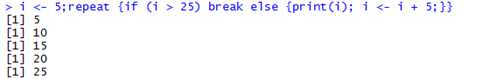
在R中有三种不同的循环结构,最简单的是repeat,仅仅简单的重复相同的表达式
repeat expression
阻止repeat,使用关键字break;跳到循环中的下一次迭代,使用next命令。例如:
> i <- 5
> repeat {if (i > 25) break else {print(i); i <- i + 5;}}
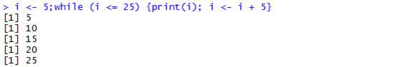
另外一个循环结构是while循环,which repeat an expression while a condition
is true。
while (condition) expression
> i <- 5;while (i <= 25) {print(i); i <- i + 5}
同样,可以在while循环中,使用break和next。
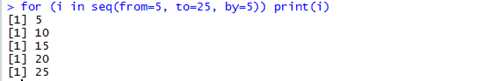
最后,便是for循环,which iterate through each item in a vector (or a list):
for (var in list) expression
例子
> for (i in seq(from=5, to=25, by=5)) print(i)
同样,可以在for循环中使用break和next函数
关于循环语句,有两点需要谨记。一是:除非你调用print函数,否则结果不会打印输出,例如
> for (i in seq(from=5, to=25, by=5)) i

二是:the variable var that is set in a for loop is changed in the calling environment
和条件语句一样,循环函数:repeat,while和for的类型都是special,因为expression is not necessarily evaluated。
很遗憾,R未提供iterators和foreach循环。但是可以通过附加包(add-on packags)来完成此功能。
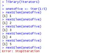
对于iterators,安装iterators包,Iterators can return elements of a vector, array, data frame, or other object。
格式:iter(obj, checkFunc=function(...) TRUE, recycle=FALSE,...)
参数obj指定对象,recycle指定当它遍历完元素时iterator是否应该重置(reset)。如果下一个值匹配checkFunc,该值被返回,否则函数会继续尝试其他值。NextElem将会check values直到它找到匹配checkFunc的值或它run out of values。When there are no elements left, the iterator calls stop with the message "StopIteration."。例如,创建一个返回1:5之间的一个迭代器。
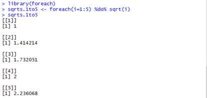
第二个便是foreach循环,需要加载foreach包。Foreach provides an elegant way to loop through multiple elements of another object (such as a vector, matrix, data frame, or iterator), evaluate an expression for each element, and return the results.下面是foreach函数的原型。
foreach(..., .combine, .init, .final=NULL, .inorder=TRUE,
.multicombine=FALSE,
.maxcombine=if (.multicombine) 100 else 2,
.errorhandling=c(‘stop‘, ‘remove‘, ‘pass‘),
.packages=NULL, .export=NULL, .noexport=NULL,
.verbose=FALSE)
Foreach函数返回一个foreach对象,为了对循环估值(evaluate),需要将foreach循环运用到一个R表达式中(使用%do% or %dopar%操作符)。例如,使用foreach循环来计算1:5数值的平方根。
The %do% operator evaluates the expression in serial, while the %dopar% can be used
to evaluate expressions in parallel。
You can fetch items by location within a data structure or by name.
@ 数据结构运算符
Table 6-2 shows the operators in R used for accessing objects in a data structure.
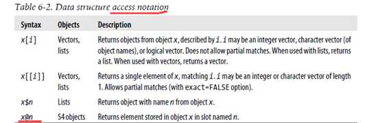
知识点:单方括号和双方括号的区别
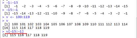
@ 通过整数向量索引(Indexing by Integer Vector)
例子
> v <- 100:119
> v[5]
[1] 104
> v[1:5]
[1] 100 101 102 103 104
> v[c(1, 6, 11, 16)]
[1] 100 105 110 115
特别地,可以使用双方框括号来reference单个元素(在该例中,作用于single bracket一样)
> v[[3]]
[1] 102
还可以使用负整数来返回一个向量包含出了指定元素的所有元素的向量
> # exclude elements 1:15 (by specifying indexes -1 to -15)
> v[-15:-1]
[1] 115 116 117 118 119
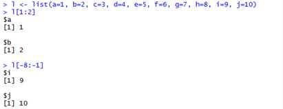
向量的符号同样适用于列表
 多维数据结构,同样也使用,如matrix,array等,对于矩阵
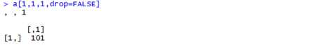
对于数组
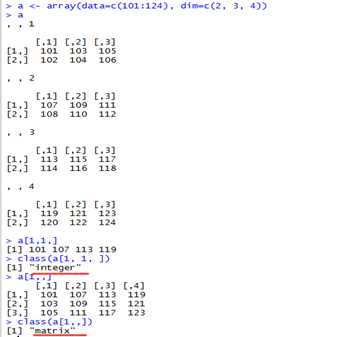
取子集时,R会自动强转结果为最合适的维数,If you select a subset of elements that corresponds to a matrix, R will return a matrix object; if you select a subset that corresponds to only a vector, R will return a vector object,To disable(禁用) this behavior, you can use the
drop=FALSE option。
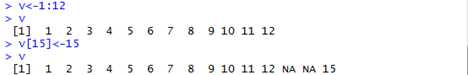
甚至可以使用这种符号扩展数据结构。A special NA element is used to represent values that are not defined:
@通过逻辑向量索引(Indexing by Logical Vector)
例如
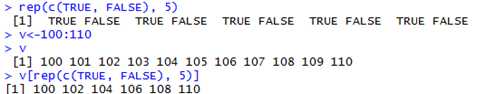
通常,it is useful to calculate a logical vector from the vector itself。
> # trivial example: return element that is equal to 103
> v[(v==103)]
> # more interesting example: multiples of three
> v[(v %% 3 == 0)]
[1] 102 105 108 111 114 117
需要注意的是,索引向量不必和向量本身长度一样,R会将短向量重复,并返回匹配值。

@通过名称索引(Indexing by Name)
在列表,可以使用名称来索引元素
> l <- list(a=1, b=2, c=3, d=4, e=5, f=6, g=7, h=8, i=9, j=10)
> l$j
[1] 10
> l[c("a", "b", "c")]
$a
[1] 1
$b
[1] 2
$c
[1] 3
可以使用双方括号进行索引,甚至还可以进行部分匹配(将参数设置为:exact=FALSE)
> dairy <- list(milk="1 gallon", butter="1 pound", eggs=12)
> dairy[["milk"]]
[1] "1 gallon"
> dairy[["mil",exact=FALSE]]
[1] "1 gallon"
In this book, I‘ve tried to stick to Google‘s R Style Guide, which is available at http://google-styleguide.googlecode.com/svn/trunk/google-r-style.html 。 Here is a summary
of its suggestions:
Indentation
Indent lines with two spaces, not tabs. If code is inside parentheses, indent to
the innermost parentheses.
Spacing
Use only single spaces. Add spaces between binary operators and operands. Do
not add spaces between a function name and the argument list. Add a single
space between items in a list, after each comma.
Blocks
Don‘t place an opening brace ("{") on its own line. Do place a closing brace
("}") on its own line. Indent inner blocks (by two spaces).
Semicolons
Omit semicolons at the end of lines when they are optional.
Naming
Name objects with lowercase words, separated by periods. For function names,
capitalize the name of each word that is joined together, with no periods. Try
to make function names verbs.
Assignment
Use <-, not = for assignment statements
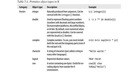
Basic vectors
These are vectors containing a single type of value: integers, floating-point
numbers, complex numbers, text, logical values, or raw data.
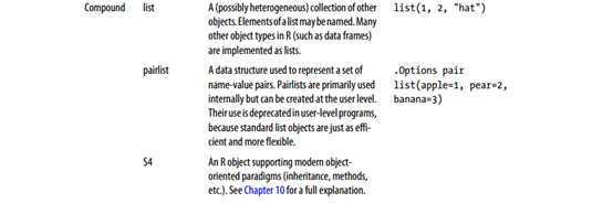
Compound objects
These objects are containers for the basic vectors: lists, pairlists, S4 objects, and
environments. Each of these objects has unique properties (described below),
but each of them contains a number of named objects.
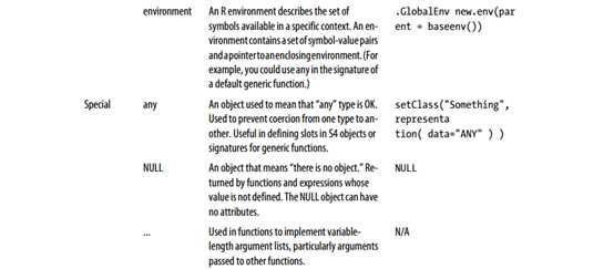
Special objects
These objects serve a special purpose in R programming: any, NULL, and ... .
Each of these means something important in a specific context, but you would
never create an object of these types.
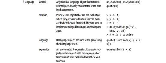
R language
These are objects that represent R code; they can be evaluated to return other
Objects.
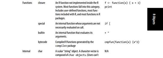
Functions
Functions are the workhorses of R; they take arguments as inputs and return
objects as outputs. Sometimes, they may modify objects in the environment or
cause side effects outside the R environment like plotting graphics, saving files,
or sending data over the network.
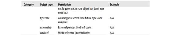
Internal
These are object types that are formally defined by R but which aren‘t normally
accessible within the R language. In normal R programming, you will probably
never encounter any of the objects.
Bytecode Objects
If you use the bytecode compiler, R will generate bytecode objects that run on
the R virtual machine.
使用R,会遇到六种六种基本的向量类型。R包括几种创建一个新向量的不同方式,最简单的是C函数(将其中的参数合并成一个向量)
> # a vector of five numbers
> v <- c(.295, .300, .250, .287, .215)
> v
[1] 0.295 0.300 0.250 0.287 0.215
C函数可以将所有的参数强转成单一类型
> # creating a vector from four numbers and a char
> v <- c(.295, .300, .250, .287, "zilch")
> v
[1] "0.295" "0.3" "0.25" "0.287" "zilch"
使用recursive=TRUE参数,可以将其他数据结构数据合并成一个向量
> # creating a vector from four numbers and a list of three more
> v <- c(.295, .300, .250, .287, list(.102, .200, .303), recursive=TRUE)
> v
[1] 0.295 0.300 0.250 0.287 0.102 0.200 0.303
注意到,使用一个list作为参数,返回的会是一个list,如下
> v <- c(.295, .300, .250, .287, list(.102, .200, .303), recursive=TRUE)
> v
[1] 0.295 0.300 0.250 0.287 0.102 0.200 0.303
> typeof(v)
[1] "double"
> v <- c(.295, .300, .250, .287, list(1, 2, 3))
> typeof(v)
[1] "list"
> class(v)
[1] "list"
另外一个组装向量的有用工具是":"运算符。这个运算符从第一个算子(operand)到第二个算子创建值序列。
> 1:10
[1] 1 2 3 4 5 6 7 8 9 10
更加灵活的方式是使用seq函数
> seq(from=5, to=25, by=5)
[1] 5 10 15 20 25
对于向量,我们可以通过length属性操纵一个向量的长度。
> w <- 1:10
> w
[1] 1 2 3 4 5 6 7 8 9 10
> length(w) <- 5
> w
[1] 1 2 3 4 5
> length(w) <- 10
> w
[1] 1 2 3 4 5 NA NA NA NA NA
An R list is an ordered collection of objects(略)
@矩阵(matrices)
A matrix is an extension of a vector to two dimensions。A matrix is used to represent two-dimensional data of a single type
生成矩阵的函数是matrix。
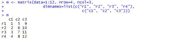
可以使用as.matrix函数将其他数据结构转换成一个矩阵。不同于其他类,矩阵没有显式类属性!
@数组(arrays)
An array is an extension of a vector to more than two dimensions。Arrays are used to represent multidimensional data of a single type。
生成数组用array函数。
同样,arrays don‘t have an explicit class attribute!
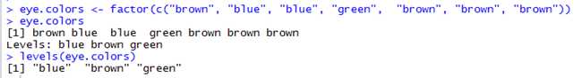
@因子(factors)
A factor is an ordered collection of items. The different values that the factor can take are called levels.
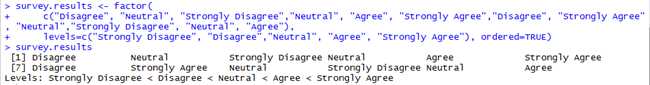
在眼睛颜色的例子中,顺序不重要,但是有些时候,因子的顺序是事关重要的。例如,在一次调查中,你调查受试者对下面这句话的感觉:melon is delicious with an omelet,受试者可以给出以下几种回答:Strongly Disagree, Disagree, Neutral, Agree, Strongly Agree.
R中有很多方式来表示这种情况,一是可以将这些编码成整数,on a scale of 5.但是这种方式有缺点,例如: is the difference between Strongly Disagree and Disagree the same as the difference between Disagree and Neutral? Can you be sure that a Disagree response and an Agree response
average out to Neutral?
为了解决这个问题,可以使用有序的因子来代表这些受试者的回答,例如
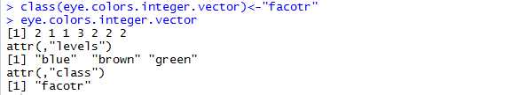
因子使用整数进行内部实施。The levels attribute maps each integer to a factor level
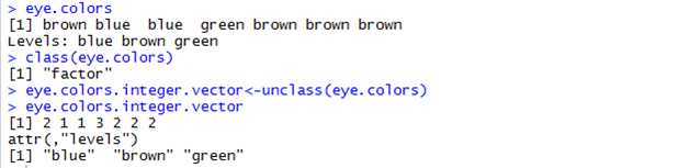
通过设置类属性,可以将这个转变成一个因子。
数据框是一种代表表格数据的有用方式。A data frame represents a table of data. Each column may be a different type, but each row in the data frame must have the same length
数据的格式如下
R provides a formula class that lets you describe the relationship。下面来创建一个公式
Here is an explanation of the meaning of different items in formulas:
Variable names
Represent variable names.
Tilde (~) 波浪字符
Used to show the relationship between the response variables (to the left) and
the stimulus variables (to the right).
Plus sign (+)
Used to express a linear relationship between variables.
Zero (0)
When added to a formula, indicates that no intercept term should be included.
For example:
y~u+w+v+0
Vertical bar (|)
Used to specify conditioning variables (in lattice formulas; see "Customizing
Lattice Graphics" on page 312).
Identity function (I())
Used to indicate that the enclosed expression should be interpreted by its arithmetic meaning. For example:
a+b
means that both a and b should be included in the formula. The formula:
I(a+b)
means that "a plus b" should be included in the formula.
Asterisk (*)
Used to indicate interactions between variables. For example:
y~(u+v)*w
is equivalent to:
y~u+v+w+I(u*w)+I(v*w)
Caret (^) 托字符号
Used to indicate crossing to a specific degree. For example:
y~(u+w)^2
is equivalent to:
y~(u+w)*(u+w)
Function of variables
Indicates that the function of the specified variables should be interpreted as a
variable. For example:
y~log(u)+sin(v)+w
Some additional items have special meaning in formulas, for example s() for
smoothing splines in formulas passed to gam. We‘ll revisit formulas in Chapter 14
and Chapter 20。
Many important problems look at how a variable changes over time,R包括了一个类来代表这种数据:时间序列对象(time series objects)。时间序列的回归函数(比如ar或arima)使用时间序列对象。此外,许多绘图函数都有针对时间序列的特殊方法。
创建时间序列对象(类ts),使用ts函数:
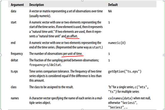
ts(data = NA, start = 1, end = numeric(0), frequency = 1,
deltat = 1, ts.eps = getOption("ts.eps"), class = , names = )
# data参数指定观测值序列;其他参数指定观测值何时be taken。下面是ts参数的描述。
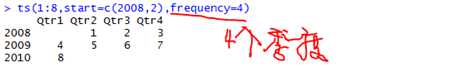
当与月或季度一起使用时,时间序列对象print方法的可以输出很好看的结果。例如:创建一个时间序列,代表2008年Q2季度到2010年Q1间的 8个连续季度。
另一个时间序列的例子,谈谈turkey价格。US农业部有一个项目,搜集各种肉制品的零售价格(retail price),该数据来自代表了约美国20%的超市,已按月和区域平均。该数据集包括在nutshell包(名称为:turkey.price.ts数据集)
> library(nutshell)
> data(turkey.price.ts)
> turkey.price.ts
Jan Feb Mar Apr May Jun Jul Aug Sep Oct Nov Dec
2001 1.58 1.75 1.63 1.45 1.56 2.07 1.81 1.74 1.54 1.45 0.57 1.15
2002 1.50 1.66 1.34 1.67 1.81 1.60 1.70 1.87 1.47 1.59 0.74 0.82
2003 1.43 1.77 1.47 1.38 1.66 1.66 1.61 1.74 1.62 1.39 0.70 1.07
2004 1.48 1.48 1.50 1.27 1.56 1.61 1.55 1.69 1.49 1.32 0.53 1.03
2005 1.62 1.63 1.40 1.73 1.73 1.80 1.92 1.77 1.71 1.53 0.67 1.09
2006 1.71 1.90 1.68 1.46 1.86 1.85 1.88 1.86 1.62 1.45 0.67 1.18
2007 1.68 1.74 1.70 1.49 1.81 1.96 1.97 1.91 1.89 1.65 0.70 1.17
2008 1.76 1.78 1.53 1.90
R包含了许多查看时间序列对象的有用函数
> start(turkey.price.ts)
[1] 2001 1
> end(turkey.price.ts)
[1] 2008 4
> frequency(turkey.price.ts)
[1] 12
> deltat(turkey.price.ts) # 不懂啊 deltat=1/frequency=1/12=
[1] 0.08333333
A shingle is a generalization of a factor to a continuous variable。A shingle consists of a numeric vector and a set of intervals。The intervals are allowed to overlap (much like roof shingles; hence the name "shingles")。Shingles在lattice包中被广泛使用。they allow you to easily use a continuous variable as a conditioning or grouping variable。
R包含了一组类来代表日期和时间
Date
Represents dates but not times.
POSIXct
Stores dates and times as seconds since January 1, 1970, 12:00 A.M.
POSIXlt
Stores dates and times in separate vectors. The list includes sec (0–61) , min
(0–59), hour (0–23), mday (day of month, 1–31), mon (month, 0–11), year
(years since 1900), wday (day of week, 0–6), yday (day of year, 0–365), and
isdst (flag for "is daylight savings time").
The date and time classes include functions for addition and subtraction。例如:
此外,R includes a number of other functions for manipulating time and date objects. Many plotting functions require dates and times.
R包括了接受或发送数据( from applications or files outside the R environment.)的特殊对象类型。可以创建到文件,URLs,zip-压缩文件,gzip-压缩文件,bzip-压缩文件,Unix pipes, network sockets,和FIFO(first in,first out)对象的连接。甚至可以从系统剪贴板(Clipboard)读取。
????为了了使用连接,我们需要创建连接,打开连接,使用连接,关闭连接。例如,在一个名为consumption的文件中保存了一些数据对象。RData想要加载该数据。R将该文件保存成了压缩文件格式。因此,我们需要创建一个与gzfile的连接。如下
> consumption.connection <- gzfile(description="consumption.RData",open="r")
> load(consumption.connection)
> close(consumption.connection)
关于连接的更多信息参考 connection帮助。
Objects in R can have many properties associated with them, called attributes. These properties explain what an object represents and how it should be interpreted by R.表7中罗列出了一些重要的属性。
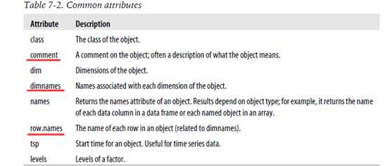
对于R,表中的查询对象属性的方式是a(X),其中a代表属性,X代表对象。使用attributes函数,可以得到一个对象的所有属性列表。例如
@查看该对象的属性
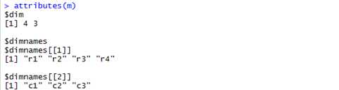
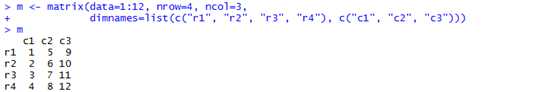
也可以直接用 dimnames(m)
@ 访问行和列名的便捷函数
> colnames(m)
[1] "c1" "c2" "c3"
> rownames(m)
[1] "r1" "r2" "r3" "r4"
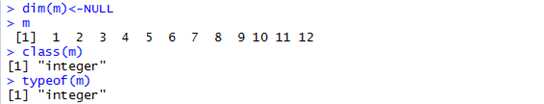
可以简单通过改变属性,将矩阵转变成其他对象。如下,移除维度属性,对象被转化成一个向量。
再看一个小知识点
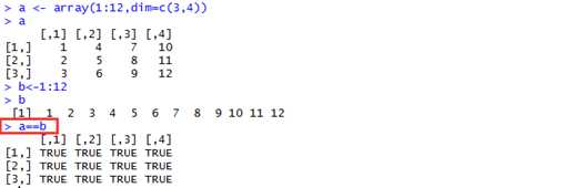
在R中,有一个all.equal函数,比较两个对象的数据和属性,返回的结果会说明是否相等,如果不相等,会给出原因,如下
> all.equal(a,b)
[1] "Attributes: < Modes: list, NULL >"
[2] "Attributes: < Lengths: 1, 0 >"
[3] "Attributes: < names for target but not for current >"
[4] "Attributes: < current is not list-like >"
[5] "target is matrix, current is numeric"
如果我们只想检查两个对象是否完全相等(exactly the same),不想知道原因,使用identical函数。如下:
> identical(a,b)
[1] FALSE
> dim(b) <- c(3,4)
> b[2,2]
[1] 5
> all.equal(a,b)
[1] TRUE
> identical(a,b)
[1] TRUE
对于简单的对象,类和类型(class and type)高度相关。对于复杂的对象,这两个是不同的。
To determine the class of an object, you can use the class function. You can determine the underlying type of object using the typeof function.例如
> x<-c(1,2,3)
> typeof(x)
[1] "double"
> class(x)
[1] "numeric"
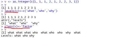
可以将一个整数数组,转变成一个因子
每一个R中的符号都定义在一个特定的环境中,An environment s an R object that contains the set of symbols available in a given context, the objects asociated with those symbols, and a pointer to a parent environment。符号和与之关联的对象被称为a frame
When R attempts to resolve a symbol, it begins by looking through the current environment. If there is no match in the local environment, then R will recursively search through parent environments looking for a match.
当你在R中定义一个变量时,实际上是在一个环境中将一个符号赋给了一个值,如下
> x <- 1
## it assigns the symbol x to a vector object of length 1 with the constant (double) value 1 in the global environment
> x <- 1
> y <- 2
> z <- 3
> v <- c(x, y, z)
> v
[1] 1 2 3
> # v has already been defined, so changing x does not change v
> x <- 10
> v
[1] 1 2 3
可以延迟一个表达式的估值(delay evaluation of an expression),因此,符号不会被立即估算,如下:
> x <- 1
> y <- 2
> z <- 3
> v <- quote(c(x, y, z))
> eval(v)
[1] 1 2 3
> x <- 5
> eval(v)
[1] 5 2 3
这一效果还可以通过创建一个promise对象来完成。使用delayedAssign函数
> x <- 1
> y <- 2
> z <- 3
> delayedAssign("v", c(x, y, z))
> x <- 5
> v
[1] 5 2 3
Promise objects are used within packages to make objects available to users without
loading them into memory
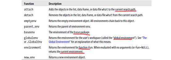
R环境也是一个对象。Table 8-1 shows the functions in R for manipulating environment objects。
显示当前环境可以用的对象集(more precisely,the set of symbols in the current environment associated with object),使用objects函数。
> x<-1
> y<-2
> z<-3
> objects()
[1] "a" "b" "m" "v" "x" "y" "z"
可以使用rm函数从当前环境中移除一个对象。
> rm(x)
> objects()
[1] "a" "b" "m" "v" "y" "z"
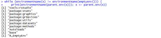
When a user starts a new session in R, the R system creates a new environment for objects created during that session. This environment is called the global environment. The global environment is not actually the root of the tree of environments. It‘s actually the last environment in the chain of environments in the search path. Here‘s the list of parent environments for the global environment in my R installation。
每一个环境都有一个父环境,除了空环境(empty environment),
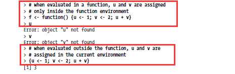
函数中局部函数与全局环境,这个好理解(略)
@@@ Working with the Call Stack
R maintains a stack of calling environments. (A stack is a data structure in which objects can be added or subtracted from only one end. Think about a stack of trays in a cafeteria; you can only add a tray to the top or take a tray off the top. Adding an object to a stack is called "pushing" the object onto the stack. Taking an object off of the stack is called "popping" the object off the stack.) Each time a new function is called, a new environment is pushed onto the call stack. When R is done evaluating a function, the environment is popped off the call stack.
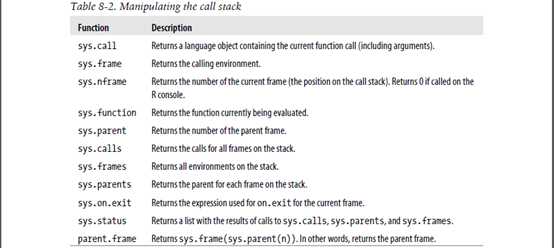
Table 8-2 shows the functions for manipulating the call stack.
@@@在不同的环境中评估函数(evaluate)
You can evaluate an expression within an arbitrary environment using the eval function:
eval(expr, envir = parent.frame(), enclos = if(is.list(envir) || is.pairlist(envir)) parent.frame() else baseenv())? |
参数说明:
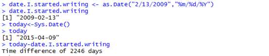
Expr:需要估算的表达式,envir:是一个估算expr的环境,数据框或pairlist;当envir是一个数据框或pairlist时,enclos就是查找对象定义的enclosure(附件/圈地)。例如
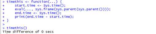
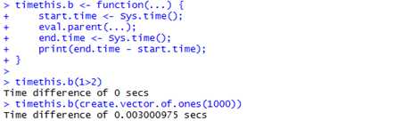
timethis <- function(...) {
start.time <- Sys.time();
eval(..., sys.frame(sys.parent(sys.parent())));
end.time <- Sys.time();
print(end.time - start.time);
}
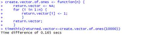
另外一个例子,我们记录将向量中的10000个元素设置为1的时间。
> create.vector.of.ones <- function(n) {
+ return.vector <- NA;
+ for (i in 1:n) {
+ return.vector[i] <- 1;
+ }
+ return.vector;
+ }
> timethis(returned.vector<-create.vector.of.ones(10000))
Time difference of 0.165 secs
这两个例子主要是想说明一个问题:eval函数在调用环境中估算一个表达式。notice that the symbol returned.vector is now defined in that environment:
> length(returned.vector)
[1] 10000
上述代码更为有效率的一种形式如下
> create.vector.of.ones.b <- function(n) {
+ return.vector <- NA;
+ length(return.vector) <- n;
+ for (i in 1:n) {
+ return.vector[i] <- 1;
+ }
+ return.vector;
+ }
> timethis(returned.vector <- create.vector.of.ones.b(10000))
Time difference of 0.04076099 secs
三种有用的简约表达式(shorthands)是evalq, eval.parent, and local。当想要引用表达式时,使用evalq,它等价于eval(quote(expr), ...);当要想在父环境中评估一个表达式时,使用eval.parent函数,等价于eval(expr, parent.frame(n));当想要在一个新的环境中评估一个表达式时,使用local函数,等价于eval(quote(expr), envir=new.env()).
下面给出如何使用eval.parent函数的例子。
start.time <- Sys.time();
eval.parent(...);
end.time <- Sys.time();
print(end.time - start.time);
}
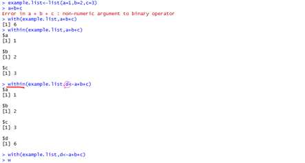
有时候,将数据框或列表当成一个环境是很方便的,这允许你通过名称来检索数据框或列表中的每一项,R使用with函数和within函数。
with(data, expr, ...) #评估表达式,返回结果
within(data, expr, ...) #在对象数据中作调整和改变,并返回结果。
The argument data is the data frame or list to treat as an environment, expr is the expression, and additional arguments in ... are passed to other methods.例子如下
@@@ Adding Objects to an Environment
Attach与detach
attach(what, pos = 2, name = deparse(substitute(what)),
warn.conflicts = TRUE)
detach(name, pos = 2, unload = FALSE)
参数
The argument what is the object to attach (called a database), pos specifies the position in the search path in which to attach the element within what, name is the name to use for the attached database (more on what this is used for below), warn.conflicts specifies whether to warn the user if there are conflicts.
you can use attach to load all the elements specified within a dataframe or list into the current environment
使用attach时要注意,因为环境中有相同的命名列时,会confusing,所以It is often better to use functions like transform to change values within a data frame or with to evaluate expressions using values in a data frame.
也许,你会发现,当你输入无效的表达式时,R会给出错误提示,例如
> 12 / "hat"
Error in 12/"hat" : non-numeric argument to binary operator
有时候,会给出警告提示.。这部分解释错误处理体系(error-handling system)的运行机制。
@@@signaling errors(发出错误提示!!!)
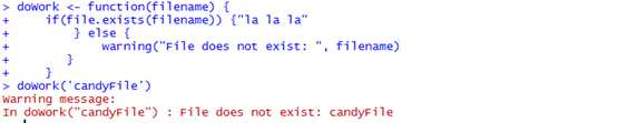
If something occurs in your code that requires you to stop execution, you can use the stop function.例如:To stop execution and print a helpful error message,you could structure your code like this。
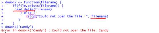
如果代码中发生了你想要告诉用户的something,可以使用warning函数。再看上述例子,如果文件名存在,返回"lalala",如果不存在,warn the user that the file does not exist。
如果仅仅告诉用户something,使用message函数,例如
> doNothing <- function(x) {
+ message("This function does nothing.")
+ }
> doNothing("another input value")
This function does nothing
@@@捕获错误/异常(catching errors)
使用Try函数,例子如下
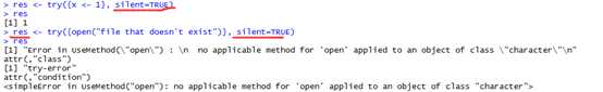
公式:Try(expr, silent) # The second argument specifies whether the error message should be printed to the R console (or stderr); the default is to print errors
#### If the expression results in an error, then try returns an object of class "try-error"
使用tryCatch函数,
公式:tryCatch(expression, handler1, handler2, ..., finally=finalexpr)
##### an expression to try, a set of handlers for different conditions, and a final expression to evaluate。
R解释器首先会估算expression,如果条件发生(an error 或 warning),R会选择针对该条件合适的处理器(handler),在expression会估算之后,评估finalexpr。(The handlers will not be active when this expression is evaluated)
Functions are the R objects that evaluate a set of input arguments and return an output value。
在R中,R对象如下定义:function(arguments) body,例如
f <- function(x,y) x + y
f <- function(x,y) {x + y}
1)参数可能包括默认值。If you specify a default value for an argument, then the argument is considered optional:
> f <- function(x, y) {x + y}
> f(1,2)
[1] 3
> g <- function(x, y=10) {x + y}
> g(1)
[1] 11
如果不指定参数的默认值,使用该参数时会报错。
2)在R中,在参数中使用ellipsis(…)来完成给其他函数传递额外的参数,例如:
创建一个输出第一个参数的函数,然后传递所有的其他参数给summary函数。
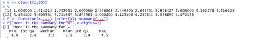
Notice that all of the arguments after x were passed to summary.
3)可以从变量-长度参数列表中读取参数。这需要将…对象转变成函数体中的一个列表。例如:
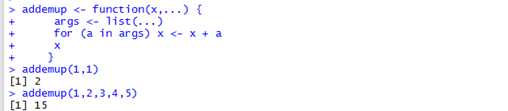
You can also directly refer to items within the list ... through the variables ..1, ..2, to ..9. Use ..1 for the first item, ..2 for the second, and so on. Named arguments are valid symbols within the body of the function。
使用return函数来指定函数的返回值
> f <- function(x) {return(x^2 + 3)}
> f(3)
[1] 12
然而,R会简单地将最后一个估算表达式作为函数结果返回,通常return可以省略
> f <- function(x) {x^2 + 3}
> f(3)
[1] 12
例如
> a <- 1:7
> sapply(a, sqrt)
[1] 1.000000 1.414214 1.732051 2.000000 2.236068 2.449490 2.645751
@@@@匿名函数
目前为止,我们看到的都是命名函数。it is possible to create functions that do not have names. These are called anonymous functions。Anonymous functions are usually passed as arguments to other functions。例如:
> apply.to.three <- function(f) {f(3)}
> apply.to.three(function(x) {x * 7}) #匿名函数.
[1] 21
实际上,R进行了如下操作:f= function(x) {x * 7},然后, 评估f(3),x=3;最后评估3*7=21.
又例如:
> a <- c(1, 2, 3, 4, 5)
> sapply(a, function(x) {x + 1})
[1] 2 3 4 5 6
@@@@函数属性(properties of functions)
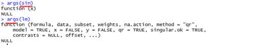
1)R包括了很多关于函数对象的函数,比如,查看一个函数接受的参数集,使用args函数,例
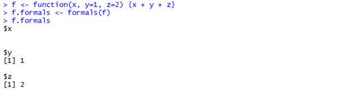
2)如果想要使用R代码来操作参数列表,可以使用formals函数,formals函数会返回一个pairlist对象(with a pair for every argument)。The name of each pair will correspond to each argument
name in the function。当定义了默认值,pairlist中的相应值会被设置为该默认值,未定义则为NULL。Formals函数仅仅可用于closure类型的对象。例如:下面是使用formals提取函数参数信息的简单例子。
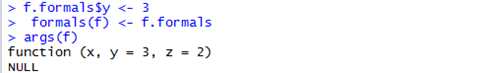
You may also use formals on the left-hand side of an assignment statement to change the formal argument for a function。例如:
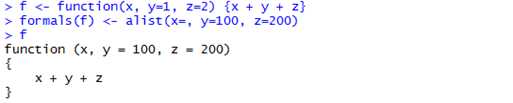
3)使用alist函数构建参数列表,alist指定参数列表就像是定义一个函数一样。(Note that for an
argument with no default, you do not need to include a value but still need to include the equals sign),例如:
4)使用body函数返回函数体
> body(f)
{
x + y + z
}
和formals函数一样,body函数可以用在赋值语句的左边。
> f
function (x, y = 3, z = 2)
{
x + y + z
}
> body(f) <- expression({x * y * z})
> f
function (x, y = 3, z = 2)
{
x * y * z
}
Note that the body of a function has type expression, so when you assign a new value it must have the type expression.
(略)
All functions in R return a value. Some functions also do other things: change variables in the current environment (or in other environments), plot graphics, load or save files, or access the network. These operations are called side effects。
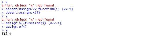
<<-运算符会causes side effects。形式如下:var <<- value。
This operator will cause the interpreter to first search through the current environment to find the symbol var。If the interpreter does not find the symbol var in the current environment, then the interpreter will next search through the parent environment. The interpreter will recursively search through environments until it either finds the symbol var or reaches the global environment。If it reaches the global environment before the symbol var is found, then R will assign value to var in the global environment。下面是一个比较<-赋值运算符和<<运算符的例子:
@@@@输入/输出
R does a lot of stuff, but it‘s not completely self-contained. If you‘re using R, you‘ll probably want to load data from external files (or from the Internet) and save data to files. These input/output (I/O) actions are side effects, because they do things other than just return an object. We‘ll talk about these functions extensively in Chapter 11.
@@@@图形
Graphics functions are another example of side effects in R. Graphics functions may return objects, but they also plot graphics (either on screen or to files). We‘ll talk about these functions in Chapters 13 and 14.
?
This part of the book explains how to accomplish some common tasks with R: loading data, transforming data, and saving data. These techniques are useful for any type of data that you want to work with in R。
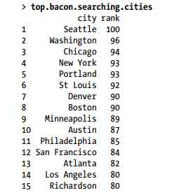
方式一:直接输入(适合小数据,比如用于测试)
方式二:edit(打开GUI),格式:var<-edit(var),简化形式直接使用fix函数(fix(var))
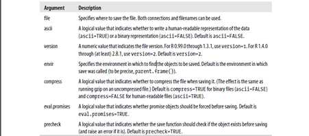
保存:save函数, save(filename, file="~/top.5.salaries.RData") #将filename保存到file指定的路径。
#####格式:
save(..., list =, file =, ascii =, version =, envir =,compress =, eval.promises =, precheck = )
参数说明
加载:load函数, load("~/top.5.salaries.RData") #加载数据
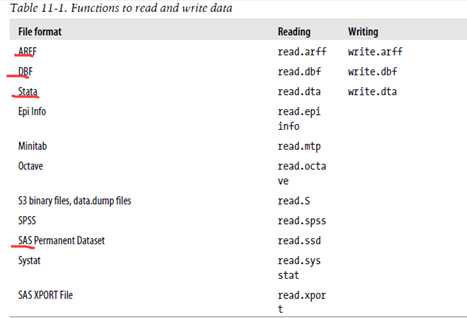
@@@文本格式text files
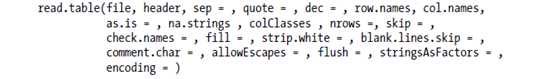
R includes a family of functions for importing delimited text files into R, based on the read.table function
|
读取text files到R中,返回一个数据框对象。每一行被解释成an observation, 每一列被解释成a variable. Read.table函数假设每一个字段都被一个分隔符(delimiter)分隔。
#####(1)例如,对于如下形式的CSV文件
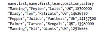
The first row contains the column names.? Each text field is encapsulated in quotes.? Each field is separated by commas。如何读取呢?
> top.5.salaries <- read.table("top.5.salaries.csv", header=TRUE, sep=",", quote="\"") #header=TRUE指定第一行为列名, sep=","指定分隔符为逗号(comma),quote="\""指定字符值使用双引号"括起来的(encapsulated)!read.table函数相当灵活,下面是关于它的参数简要说明
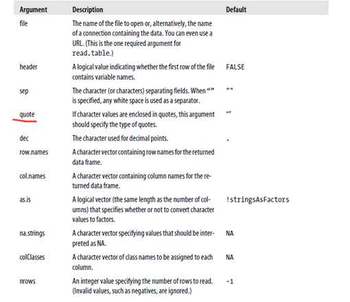
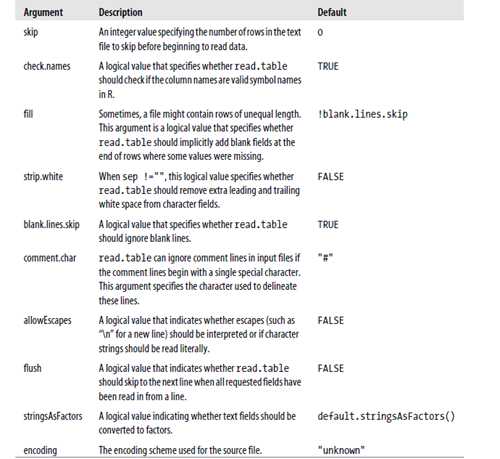
其中最重要的参数(options)是sep和header。R包括了许多调用read.table函数(不同的默认值)的便捷函数,如下
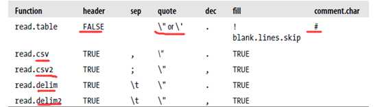
因此,大多数时候,不需要指定其他参数,就可以使用read.csv函数读取逗号分隔的稳健,read.delim读取tab分隔的文件。
#######(2)又例如,假设要分析历史股票交易数据,Yahoo!Finance提供了这方面的信息。例如,提取1999年4月1日到2009奶奶4月1日间每个月的标准普尔500指数的收盘价。数据链接地址如下 :URL<-http://ichart.finance.yahoo.com/table.csv?s=%5EGSPC&a=03&b=1&c=1999&d=03&e=1&f=2009&g=m&ignore=.csv.
>sp500 <- read.csv(paste(URL, sep=""))
> # show the first 5 rows
> sp500[1:5,]
Date Open High Low Close Volume Adj.Close
1 2009-04-01 793.59 813.62 783.32 811.08 12068280000 811.08
2 2009-03-02 729.57 832.98 666.79 797.87 7633306300 797.87
3 2009-02-02 823.09 875.01 734.52 735.09 7022036200 735.09
4 2009-01-02 902.99 943.85 804.30 825.88 5844561500 825.88
5 2008-12-01 888.61 918.85 815.69 903.25 5320791300 903.25
?如果,知道需要加载的文件的很大,可以使用nrows=参数来指定加载前20行用于测试语句的对错,测试成功后,便可全部加载!!!
2)固定宽度的文件
读取固定宽度的text文件,使用read.fwf函数,格式如下:

下面是该函数的参数说明
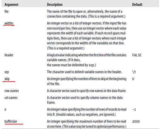
注意:read.fwf还可以接收read.table使用的参数,包括as.is, na.strings, colClasses, and strip.white。
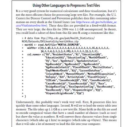
因此,建议使用脚本语言,比如Perl,Python,Ruby先将大而复杂的文本文件处理成R容易理解的形式(digestible form.)。
3)其他解析数据的函数
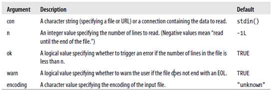
####To read data into R one line at a time, use the function readLines:

参数描述
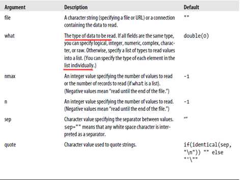
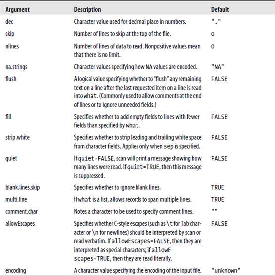
##### Another useful function for reading more complex file formats is scan:
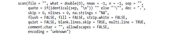
Unlike readLines,scan allows you to read data into a specifically defined data structure using the argument what.
参数说明
注意:Like readLines, you can also use scan to enter data directly into R.
@@@@其他函数
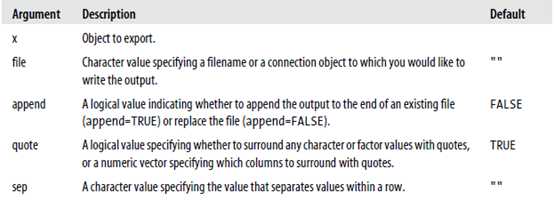
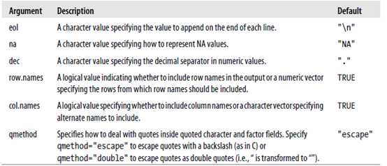
To export data to a text file, use the write.table function:
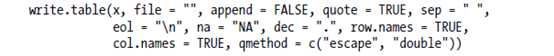
There are wrapper functions for write.table that call write.table with different defaults

下面是参数说明
One of the best approaches for working with data from a database is to export the data to a text file and then import the text file into R。
There are two sets of database interfaces available in R
? RODBC. The RODBC package allows R to fetch data from ODBC (Open DataBase Connectivity) connections. ODBC provides a standard interface for different programs to connect to databases.
? DBI. The DBI package allows R to connect to databases using native database drivers or JDBC drivers. This package provides a common database abstraction for R software. You must install additional packages to use the native drivers for each database.
对于提供的两种连接方式,如何选择呢?到底选哪一个好呢?下面给出一些标准作为参考

For this example, we will use an SQLite database containing the Baseball Databank database. You do not need to install any additional software to use this database. This file is included in the nutshell package. To access it within R, use the following expression as a filename: system.file("extdata", "bb.db", package = "nutshell").
getting RODBC working
在使用RODBC之前,需要配置ODBC连接。这个只需配置一次。
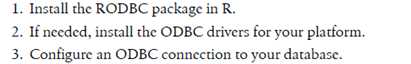
#####安装RODBC包
> install.packages("RODBC")
> library(RODBC)
#####安装ODBC驱动器
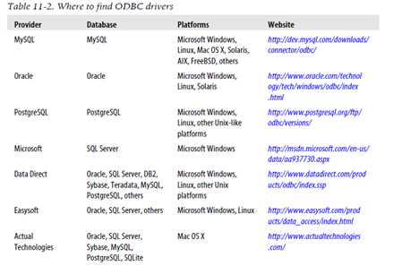
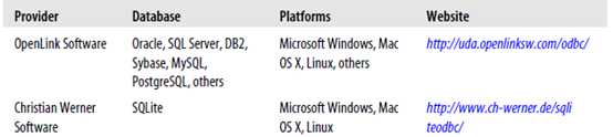
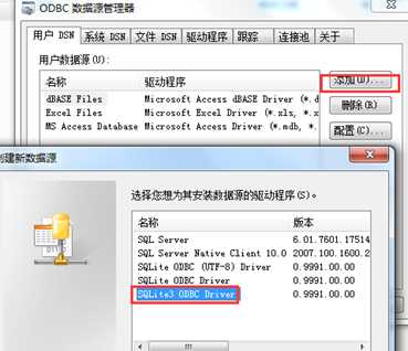
@ 对于Window用户,安装SQLite ODBC的过程如下
(原文如下)

我的安装过程:
Step1: 下载SQLite ODBC Driver, 地址http://www.ch-werner.de/sqliteodbc/

Step2:安装,默认next即可
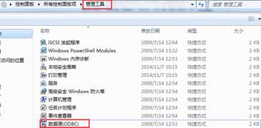
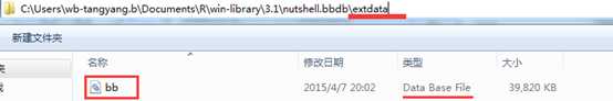
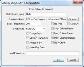
Step3:为数据库配置DSN(Distributed Service Network),打开管理工具à数据源(ODBC)-à用户DSN标签界面中选择添加,选择SQLite3 ODBC驱动,进入 SQLite3 ODBC DSN配置界面,填写数据源名称, 这里填写"bbdb";填写数据库名称,这里找到nutshell包下的exdata文件下dd数据库文件。操作过程的截图如下:
######打开管理工具,选择数据源
注意:使用如下命令可以查看一个包的完整路径名称!
> system.file(package="nutshell")
[1] "C:/Users/wb-tangyang.b/Documents/R/win-library/3.1/nutshell"
######进入ODBC数据源管理器界面,选择添加SQLite3 ODBC Driver.
#####弹出SQLite3 ODBC DSN 配置界面,填写相关信息
?
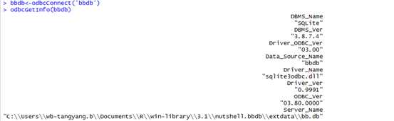
@@@@@这样ODBC驱动就配置好啦!下面来通过ODBC访问bbdb文件. 在R中使用如下命令来检查ODBC配置是否运行正常。
> bbdb<-odbcConnect(‘bbdb‘)
> odbcGetInfo(bbdb)
Connecting to a database in R is like connecting to a file. First, you need to connect to a database. Next, you can execute any database queries. Finally, you should close the connection.
######打开一个channel(连接)
To establish a connection, use the odbcConnect function。
odbcConnect(dsn, uid = "", pwd = "", ...)
You need to specify the DSN for the database to which you want to connect. If you did not specify a username and password in the DSN, you may specify a username with the uid argument and a password with the pwd argument. Other arguments are passed to the underlying odbcDriverConnect function. The odbcConnect function returns an object of class RODBC that identifies the connection. This object is usually called a channel.
下面是使用该函数连接"bbdb"DSN的例子。
> library(RODBC)
> bbdb <- odbcConnect("bbdb")
#####获取数据库中的信息(get information about the database)
You can get information about an ODBC connection using the odbcGetInfo function.
This function takes a channel (the object returned by odbcConnect) as its only argument. It returns a character vector with information about the driver and connection;
为了得到基本数据库(underlying database)中的表列表,使用sqlTables function。This function returns a data frame with information about the available tables。
> sqlTables(bbdb) # 因为表中没有数据!!!
[1] TABLE_CAT TABLE_SCHEM TABLE_NAME TABLE_TYPE REMARKS
<0 行> (或0-长度的row.names)
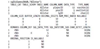
获取一个特定表中列的详细信息,使用sqlColumns function。
######获取数据(getting data)
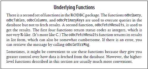
Finally, we‘ve gotten to the interesting part: executing queries in the database and returning results. RODBC provides some functions that let you query a database even if you don‘t know SQL。
从基本数据库中获取一个表或试图,使用sqlFetch function. This function returns a data frame containing the contents of the table。
sqlFetch(channel, sqtable, ..., colnames = , rownames = )
> teams <- sqlFetch(bbdb,"Teams")
> names(teams)
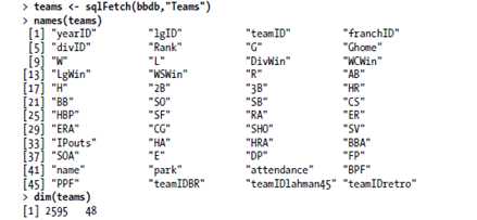
After loading the table into R, you can easily manipulate the data using R commands
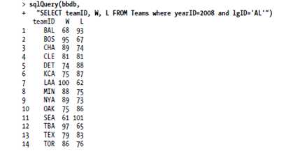
You can also execute an arbitrary SQL query in the underlying database,使用sqlQuery function:
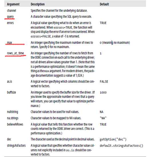
sqlQuery(channel, query, errors = , max =, ..., rows_at_time = )
如果想要从一个很大的表中获取数据,建议不要一次性获取所有的数据。RODBC库提供了分段获取结果的机制(fetch results piecewise)。首先,调用sqlQuery或sqlFetch函数, 但是需要指定一个max值,告诉函数,每一次要想获取(retrieve)的最大行数。可以通过sqlGetResults函数获取剩下的行!
sqlGetResults(channel, as.is = , errors = , max = , buffsize = ,
nullstring = , na.strings = , believeNRows = , dec = ,
stringsAsFactors = )
实际上,sqlQuery函数就是调用的sqlGetResults函数来获取查询的结果的。下面是这两个函数的参数列表((If you are using sqlFetch, the corresponding function to fetch additional rows is sqlFetchMore)。
By the way, notice that the sqlQuery function can be used to execute any valid query in the underlying database. It is most commonly used to just query results (using SELECT queries), but you can enter any valid data manipulation language query (including SELECT, INSERT, DELETE, and UPDATE queries) and data definition language query (including CREATE, DROP, and ALTER queries).
?
?
######关闭一个channel(通道)
When you are done using an RODBC channel, you can close it with the odbcClose function. This function takes the connection name as its only argument:
> odbcClose(bbdb)
Conveniently, you can also close all open channels using the odbcCloseAll function. It is generally a good practice to close connections when you are done, because this frees resources locally and in the underlying database.
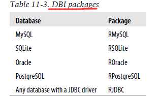
One important difference between the DBI packages and the RODBC package is in the objects they use: DBI uses S4 objects to represent drivers, connections, and other objects
Table 11-3 shows the set of database drivers available through this interface
安装和加载RSQLite包
> install.packages("RSQLite")
> library(RSQLite)
If you are familiar with SQL but new to SQLite, you may want to review what SQL commands are supported by SQLite. You can find this list at http://www.sqlite.org/lang.html.
打开连接
To open a connection with DBI, use the dbConnect function:
dbConnect(drv, ...)
获取DB信息
查询数据库
清洗(cleaning up)
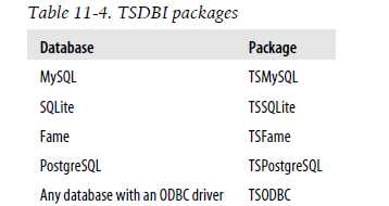
There is one last database interface in R that you might find useful: TSDBI. TSDBI is an interface specifically designed for time series data. There are TSDBI packages for many popular databases, as shown in Table 11-4.
Today, one of the most important sources for data is Hadoop. To learn more about Hadoop, including instructions on how to install R packages for working with Hadoop data on HDFS or in HBase, see "R and Hadoop" on page 549.
Everyone loves building models, drawing charts, and playing with cool algorithms. Unfortunately,
most of the time you spend on data analysis projects is spent on preparing data for analysis. I‘d estimate that 80% of the effort on a typical project is spent on finding, cleaning, and preparing data for analysis. Less than 5% of the effort is devoted to analysis. (The rest of the time is spent on writing up what you did.)
合并数据集主要用于处理存储在不同地方的数据!(类似于SQL中的各种连接!!!)
R provides several functions that allow you to paste together multiple data structures into a single structure.
这些函数中,最简单的一个就是paste函数。它将多个字符向量连接合并(concatenate)成单个向量(如果不是字符的将会首先被强转为字符.)
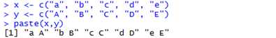
默认下,值由空格分隔,可以用sep参数指定其他的分隔符(separator)

如果想得到:返回的向量中所有的值被依次被连接,可以指定collapse参数,collapse的值会被用作这个值中的分隔符。

#### cbind函数通过添加列来合并对象,可以看成,水平地合并两个表。例如:
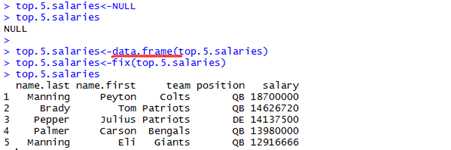
> top.5.salaries<-NULL > top.5.salaries NULL > top.5.salaries<-data.frame(top.5.salaries) > top.5.salaries<-fix(top.5.salaries) |
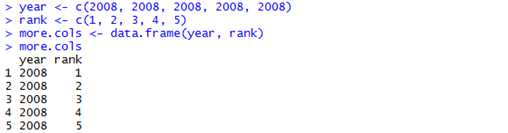
接着,创建一个两列的数据框(year和rank)。
> year <- c(2008, 2008, 2008, 2008, 2008) > rank <- c(1, 2, 3, 4, 5) > more.cols <- data.frame(year, rank)? |
 、
、
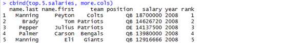
然后,合并这两个数据框:使用cbind函数
> cbind(top.5.salaries, more.cols)
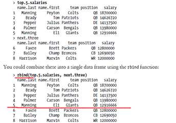
##### 同理,rbind函数通过行来合并对象,可以想象成垂直地合并两个表!
######扩展例子
To show how to fetch and combine together data and build a data frame for analysis,we‘ll use an example from the previous chapter: stock quotes. Yahoo! Finance allows you to download CSV files with stock quotes for a single ticker..
假设我们想要一个关于多只证券的股票报价的数据集(比如,DJIA中的30只股票)。我们需要将每次通过查询返回的单个数据集合并在一起。首先,写一个函数,组合URL;然后获取带内容的数据框。
这个函数的思路如下:首先,定义URL(作者通过试错法来确定了URL的格式)。使用paste函数将所有的这些字符值合在一起。然后,使用read.csv函数获取URL,将数据框赋给tmp符号。数据框有大多数我们想要的信息,但是没有ticker符号,因此,我们将会使用cbind函数附加一个ticker符号向量到数据框中。(by the way,函数使用Date对象代表日期)。 I also used the current date as the default value for to, and the date one year ago as the default value for from。具体函数如下:
URL地址示例:
http://ichart.finance.yahoo.com/table.csv?s=%5EGSPC&a=03&b=1&c=1999&d=03&e=1&f=2009&g=m&ignore=.csv
get.quotes <- function(ticker, # ticker指的是股票代号/或者代码!
from=(Sys.Date()-365), # 这里定义下载数据的时间范围:从过去一年到现在!
to=(Sys.Date()),
interval="d") { # 时间间隔,以天为单位!!!
# define parts of the URL
base <- "http://ichart.finance.yahoo.com/table.csv?"; #定义URL的主体部分!
symbol <- paste("s=", ticker, sep=""); # 股票代码符号
# months are numbered from 00 to 11, so format the month correctly
from.month <- paste("&a=",
formatC(as.integer(format(from,"%m"))-1,width=2,flag="0"), sep=""); #月, 高两部分提取日期中的月份!
from.day <- paste("&b=", format(from,"%d"), sep=""); #日
from.year <- paste("&c=", format(from,"%Y"), sep=""); #年
to.month <- paste("&d=",
formatC(as.integer(format(to,"%m"))-1,width=2,flag="0"), #formatC函数很吊啊
sep="");
to.day <- paste("&e=", format(to,"%d"), sep="");
to.year <- paste("&f=", format(to,"%Y"), sep="");
inter <- paste("&g=", interval, sep="");
last <- "&ignore=.csv";
# put together the url
url <- paste(base, symbol, from.month, from.day, from.year,
to.month, to.day, to.year, inter, last, sep="");
# get the file
tmp <- read.csv(url);
# add a new column with ticker symbol labels
cbind(symbol=ticker,tmp);
}
然后,写一个函数,返回一个包含多个证券代码的股票报价的数据框。这个函数每次针对tickers向量中的每一个ticker简单的调用get.quotes,然后将结果使用rbind函数合并在一起;
get.multiple.quotes <- function(tkrs,
from=(Sys.Date()-365),
to=(Sys.Date()),
interval="d") {
tmp <- NULL;
for (tkr in tkrs) {
if (is.null(tmp))
tmp <- get.quotes(tkr,from,to,interval)
else tmp <- rbind(tmp,get.quotes(tkr,from,to,interval))
}
tmp
}
最后,定义一个包含了DJIA指数ticker符号集的向量,并构建一个获取数据的数据框。
> dow.tickers <- c("MMM", "AA", "AXP", "T", "BAC", "BA", "CAT", "CVX",
"CSCO", "KO", "DD", "XOM", "GE", "HPQ", "HD", "INTC",
"IBM", "JNJ", "JPM", "KFT", "MCD", "MRK", "MSFT", "PFE",
"PG", "TRV", "UTX", "VZ", "WMT", "DIS")
> # date on which I ran this code
> Sys.Date()
[1] "2012-01-08"
> dow30 <- get.multiple.quotes(dow30.tickers) #get.multiple.quotes函数只需指定股票代码即可,方便啊!!!
下面比如我想要提取阿里巴巴的股票数据!只需输入:
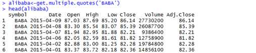
> alibaba<-get.multiple.quotes(‘BABA‘)
> head(alibaba)
symbol Date Open High Low Close Volume Adj.Close
1 BABA 2015-04-08 83.30 85.54 83.07 85.39 26087700 85.39
2 BABA 2015-04-07 81.94 82.95 81.88 82.21 9386400 82.21
3 BABA 2015-04-06 82.05 82.59 81.61 81.82 12758900 81.82
4 BABA 2015-04-02 82.88 83.00 81.25 82.28 19784800 82.28
5 BABA 2015-04-01 83.37 83.72 82.18 82.36 14856100 82.36
6 BABA 2015-03-31 83.64 84.45 83.20 83.24 11763800 83.24
 nice job!!!
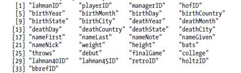
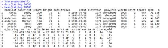
例如,回到我们在"Importing Data From Databases使用过的Baseball Databank database。在这张表中,球员的信息存储在Master表中, 并且被playerID这列唯一标识.
> dbListFields(con,"Master")
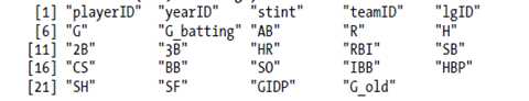
Batting信息存储在Batting表中. 球员同样被playerID这列唯一标识。
> dbListFields(con, "Batting")
假设你想要显示每一个球员(连同它的姓名和年龄)的击球统计(batting statistics). 因此, 这就需要合并两张表的数据(merge data from two tables). 在R中, 使用merge函数。
> batting <- dbGetQuery(con, "SELECT * FROM Batting")
> master <- dbGetQuery(con, "SELECT * FROM Master")
> batting.w.names <- merge(batting, master)
这样, 两张表间只有一个共同变量:playerID:
> intersect(names(batting), names(master))
[1] "playerID"
默认下,merge使用两个数据框间的共同变量作为合并的关键字(merge keys). 因此,在该案例中,我们不需要指定其他参数. 下面是merge 函数的用法说明:
merge(x, y, by = , by.x = , by.y = , all = , all.x = , all.y = ,
sort = , suffixes = , incomparables = , ...)
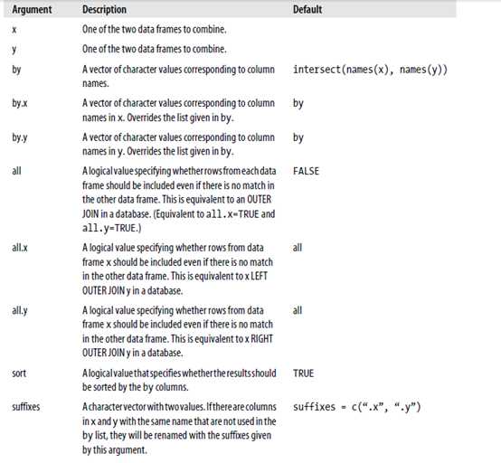

默认情况下,merge等价于SQL中的NATURAL Join。可以指定其他列来使用比如INNER JOIN。可以指定ALL参数来获得OUTER或者FULL join。If there are no matching field names,or if by is of length 0 (or by.x and by.y are of length 0), then merge will return the full Cartesian product of x and y.
?
Sometimes, there will be some variables in your source data that aren‘t quite right. This section explains how to change a variable in a data frame。
在数据框中重新定义一个变量最方便的方式是使用赋值运算符(assignment operators)。例如,假设你想要改变之前创建的alibaba数据框中一个变量的类型。当使用read.csv导入这些数据时Date字段会被解释成一个字符串,并将其转变成一个因子。
> class(alibaba$Date)
[1] "factor
Luckily, Yahoo! Finance prints dates in the default date format for R, so we can just transform these values into Date objects using as.Date函数。
> class(alibaba$Date)
[1] "factor"
> alibaba$Date<-as.Date(alibaba$Date)
> class(alibaba$Date)
[1] "Date"
当然,还可以进行其他改变,例如:define a new midpoint variable that is the mean of the high and low price。
> alibaba$mid<-(alibaba$High+alibaba$Low)/2
> names(alibaba)
[1] "symbol" "Date" "Open" "High" "Low" "Close"
[7] "Volume" "Adj.Close" "mid"
A convenient function for changing variables in a data frame is the transform function。Transform函数的定义如下:
transform(`_data`, ...)
To use transform,
you specify a data frame (as the first argument) and a set of expressions that use variables within the data frame. The transform function applies each expression to the data frame and then returns the final data frame.例如:我们通过transform函数完成上述两个任务:将Date列变成Date格式;添加一个midpoint新列。
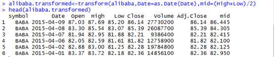
> alibaba.transformed<-transform(alibaba,Date=as.Date(Date),mid=(High+Low)/2)
> head(alibaba.transformed)
When transforming data, one common operation is to apply a function to a set of objects (or each part of a composite object) and return a new set of objects (or a new composite object
To apply a function to parts of an array (or matrix), use the apply function:
apply(X, MARGIN, FUN, ...)
Apply accepts three arguments: X is the array to which a function is applied, FUN is the function, and MARGIN specifies the dimensions to which you would like to apply a function. Optionally, you can specify arguments to FUN as addition arguments to apply arguments to FUN.)
例子1)为了展示该函数如何运作,下面给出一个简单的例子,先构建一个数据集
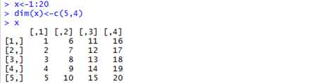
首先,使用max函数:选择每一行最大的元素。(These are the values in the rightmost column: 16, 17, 18, 19, and 20)。在apply函数中指定X=x,MARGIN=1 (rows are the first dimension), and FUN=max。
> apply(X = x,MARGIN = 1,FUN = max)
[1] 16 17 18 19 20
同样的max运用到列上面的效果如下:
> apply(X = x,MARGIN = 2,FUN = max)
[1] 5 10 15 20
例子2)再给出一个更为复杂的例子,指定margin参数,运用函数到多维数据集。如下main的一个三维数组(We‘ll switch to the function paste to show which elements were included)
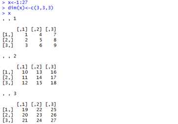
首先,looking at which values are grouped for each value of MARGIN:
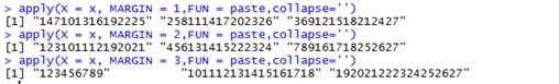
> apply(X = x, MARGIN = 1,FUN = paste,collapse=‘‘)
[1] "147101316192225" "258111417202326" "369121518212427"
> apply(X = x, MARGIN = 2,FUN = paste,collapse=‘‘)
[1] "123101112192021" "456131415222324" "789161718252627"
> apply(X = x, MARGIN = 3,FUN = paste,collapse=‘‘)
[1] "123456789" "101112131415161718" "192021222324252627"
然后,看一个更复杂的例子,Let‘s select MARGIN=c(1, 2) to see which elements are selected:
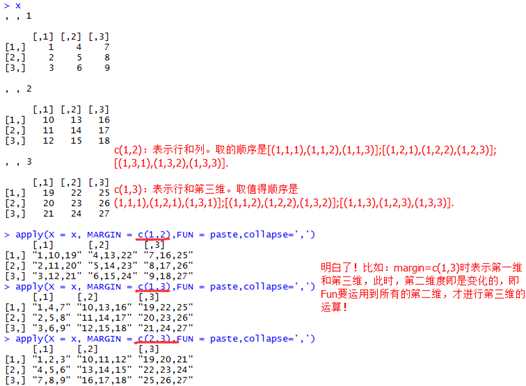
对于margin=C(1,2)时,This is the equivalent of doing the following: for each value of i between 1 and 3 and each value of j between 1 and 3, calculate FUN of x[i][j][1], x[i][j][2], x[i][j][3].
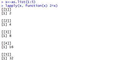
To apply a function to each element in a vector or a list and return a list, you can use the function lapply。The function lapply requires two arguments: an object X and a function FUNC. (You may specify additional arguments that will be passed to FUNC.下面看一个例子
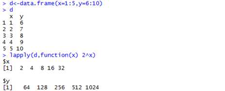
也可以对一个数据框运用一个函数,函数将会被运用到数据框中的每一个向量,例如:
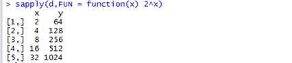
有时候,我们更喜欢返回一个向量,矩阵,或数组而不是一个列表。可以使用sapply函数,除了它返回一个向量或矩阵外,这个函数和apply函数用法相同。
另外一个相关的函数时mapply函数,是sapply的多变量版本(multivariate)!
mapply(FUN, ..., MoreArgs = , SIMPLIFY = , USE.NAMES = ),下面是mapply的参数说明
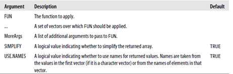
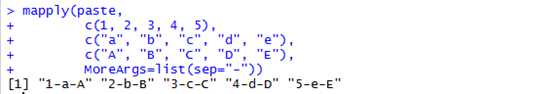
这个函数运用FUN到每一个向量的第一个元素,然后到第二个,以此类推,直到到最后一个元素。例如
mapply(paste,
+ c(1, 2, 3, 4, 5),
+ c("a", "b", "c", "d", "e"),
+ c("A", "B", "C", "D", "E"),
+ MoreArgs=list(sep="-"))
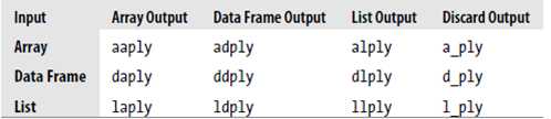
The plyr package contains a set of 12 logically named functions for applying another function to an R data object and returning the results. Each of these functions takes an array, data frame, or list as input and returns an array, data frame, list, or nothing as output。
下面是plyr库中最常用函数的列表
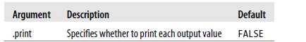
所有的这些函数接收下面的参数
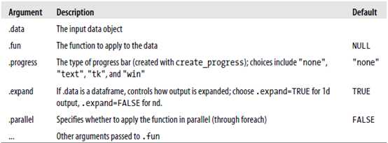
其他参数取决于输入和输出,如果输入是数组,可用参数为
如果输入是数据框,可用参数为
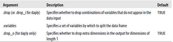
如果output is dropped,可用参数为
下面给几个例子(略),例子见plyr包学习笔记
Another common data transformation is to group a set of observations into bins based on the value of a specific variable。
例如:假设你有一些时间序列数据(以天为单位),但是你想要根据月份来汇总数据。在R中有几个可用来binning(分组/分箱)数值数据的函数。
Shingles are a way to represent intervals in R。They can be overlapping, like roof shingles(屋顶木瓦) (hence the name)。shingles在lattice包中被广泛的使用,比如,当你要想使用数值型值作为一个条件值时。
To create shingles in R, use the shingle function:
shingle(x, intervals=sort(unique(x)))
通过使用intervals参数来指定在何处分隔bins。可以使用一个数值向量来表示breaks(分割点)或一个两列的矩阵,其中每一行代表一个特定的间隔(interval)。
To create shingles where the number of observations is the same in each bin, you can use the equal.count function:
equal.count(x, ...)
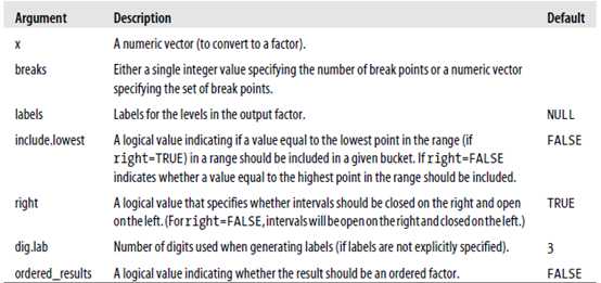
The function cut is useful for taking a continuous variable and splitting it into discrete pieces. Here is the default form of cut for use with numeric vectors:
# numeric form
cut(x, breaks, labels = NULL,
include.lowest = FALSE, right = TRUE, dig.lab = 3,
ordered_result = FALSE, ...)
另外一个操作Date对象的cut版本:
# Date form
cut(x, breaks, labels = NULL, start.on.monday = TRUE,
right = FALSE, ...)
cut函数接收一个数值向量作为输入,返回一个因子。因子中的每一个水平对应输入向量中的间隔值,下面是cut的参数描述!
例如:假设,你想要在一定范围内计算平均击球次数的球员数量,可以使用cut函数和table函数。
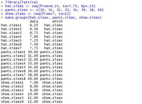
Sometimes you would like to combine a set of similar objects (either vectors or data frames) into a single data frame, with a column labeling the source.可以使用lattice包中的make.groups函数
library(lattice)
make.groups(...)
例如,合并三个不同的向量为一个数据框
hat.sizes <- seq(from=6.25, to=7.75, by=.25)
pants.sizes <- c(30, 31, 32, 33, 34, 36, 38, 40)
shoe.sizes <- seq(from=7, to=12)
make.groups(hat.sizes, pants.sizes, shoe.sizes)
One way to take a subset of a data set is to use the bracket notation。
例如,我们仅仅想要选择2008年的batting数据。Batting.w.names$ID列包含了year。因此我们写一个表达式:atting.w.names$yearID==2008,生成一个逻辑值向量,Now we just have to index the data frame batting.w.names with this vector to select only rows for the year 2008。

同样,我们可以使用同样的符号来选择某一列。Suppose that we wanted to keep only the variables nameFirst, nameLast, AB, H, and BB. We could provide these in the brackets as well:

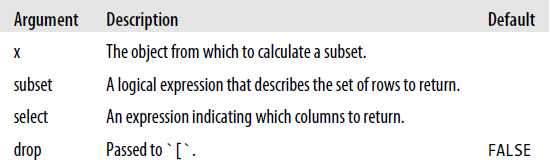
另外一种替代方案,可以使用subset函数从数据框/矩阵中对行和列取子集
subset(x, subset, select, drop = FALSE, ...)
subset函数与bracket notation的区别在于,前者会少很多代码!Subset allows you to use
variable names from the data frame when selecting subsets。下面是subset函数的参数描述:
例如:使用subset函数再做一遍上面的取子集过程
> batting.w.names.2008 <- subset(batting, yearID==2008)
> batting.w.names.2008.short <- subset(batting, yearID==2008,
+ c("nameFirst","nameLast","AB","H","BB"))
Often, it is desirable to take a random sample of a data set. Sometimes, you might have too much data (for statistical reasons or for performance reasons). Other times, you simply want to split your data into different parts for modeling (usually into training, testing, and validation subsets).
提取随机样本最简单的方式是使用sample函数。它返回一个随机的向量元素样本:
sample(x, size, replace = FALSE, prob = NULL)
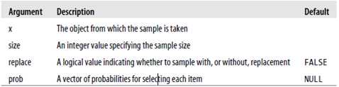
当对数据框使员工sample函数时,应该小心一点,因为,a data frame is implemented as a list of vectors, so sample is just taking a random sample of the elements of the list。return a random
sample of the columns。
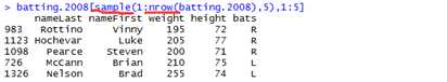
#####在实际操作中,为了对一个数据集取随机样本观测值,可以使用sample函数创建一个row numbers的随机样本,然后使用index operators来选择这些row numbers。例如:let‘s take a random sample of five elements from the batting.2008 data set。
#####还可以使用该方法来选择一个更加复杂的随机子集,例如,假设我们想要选择三个队的随机统计量。
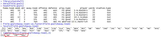
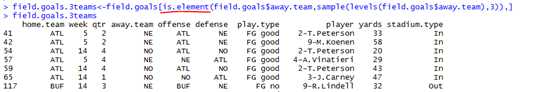
>field.goals.3teams<-field.goals[is.element(field.goals$away.team,sample(levels(field.goals$away.team),3)),]

这个函数对于仅仅要想对所有的观测值随机采样时比较有用!但是通常我们可能还想做一些更加复杂的事情,比如分层抽样(stratified sampling),聚类抽样(cluster sampling),最大熵抽样(maximum entropy sampling),或者其他复杂的方法。我们可以在sampling包中找到很多这些方法。For an example using this package to do stratified sampling, see "Machine Learning Algorithms for Classification" on page 477
假设你想要知道推送给每一个用户的平均页面数量。To find the answer,需要查看每一个HTTP transaction(对内容的每一个请求!),将所有的请求分组成一个部分(sessions),然后对请求数进行计数。
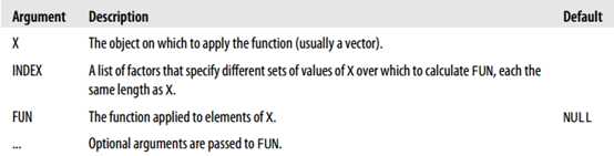
1)Tapply函数对于summarize一个向量X非常灵活。可以指定summarize向量X的哪一个子集:
tapply(X, INDEX, FUN = , ..., simplify = )
下面是tapply函数的参数
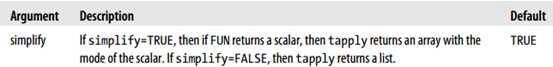
#####例如,使用tapply函数按team加总(sum)home的数量。仍然是batting.2008.rda的例子。这个数据集在包nutshell下面,运行命令:得到nutshell包所在的包路径!
> system.file(package = ‘nutshell‘)
[1] "C:/Users/wb-tangyang.b/Documents/R/win-library/3.1/nutshell"
> system.file("data",package = ‘nutshell‘)
[1] "C:/Users/wb-tangyang.b/Documents/R/win-library/3.1/nutshell/data"
然后,打开该路径,看到在data子目录下有batting.2008.rda文件,于是直接用data加载数据!
> tapply(X=batting.2008$HR, INDEX=list(batting.2008$teamID), FUN=sum)
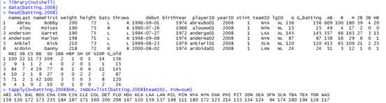
#####还可以运用返回多个项的函数,比如fivenum函数(which returns a vector containing the minimum, lower-hinge, median, upper-hinge, and maximum values)。例如,下面针对每一个球员的平均击球数(batting averages)应用fivenum函数,aggregated by league.
> tapply(X = (batting.2008$H/batting.2008$AB),INDEX = list(batting.2008$lgID),FUN = fivenum)
####还可以使用tapply函数针对多维计算summaries统计摘要。例如按照league和batting hand计算home runs per player的平均值。
> tapply(X=(batting.2008$HR),INDEX=list(batting.2008$lgID,batting.2008$bats),FUN=mean)

(注:As a side note, there is no equivalent to tapply in the plyr package)
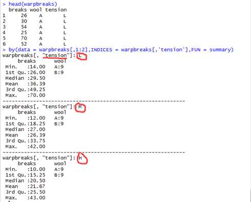
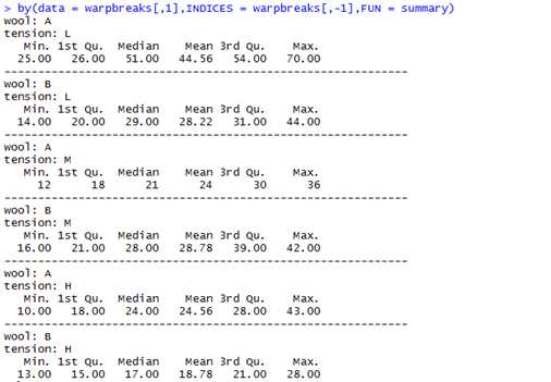
和tapply函数最相近的是by函数。唯一一点的不同是,by函数works on数据框。Tapply的index参数被indeces参数替代。
此例子来自官方文档:
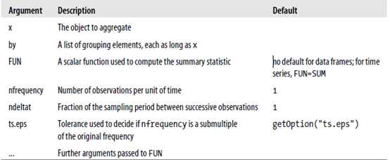
格式:aggregate(x, by, FUN, ...)
Aggregate可以被运用于时间序列,此时,参数略微有些不同
aggregate(x, nfrequency = 1, FUN = sum, ndeltat = 1,
ts.eps = getOption("ts.eps"), ...)
下面是参数说明
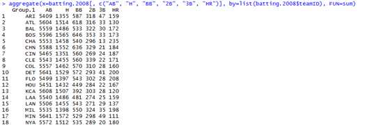
例如,we can use aggregate to summarize batting statistics by team!
> aggregate(x=batting.2008[, c("AB", "H", "BB", "2B", "3B", "HR")], by=list(batting.2008$teamID), FUN=sum)
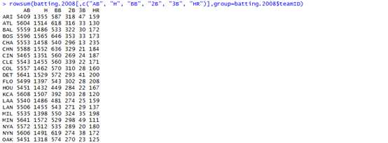
计算一个对象中某个特定变量的和(sum),通过一个分组变量(grouping variables)来分组,使用rowsum函数。
格式:rowsum(x, group, reorder = TRUE, ...)
例如:
> rowsum(batting.2008[,c("AB", "H", "BB", "2B", "3B", "HR")],group=batting.2008$teamID)
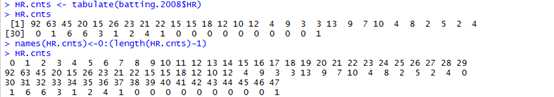
1)The simplest function for counting the number of observations that take on a value is the tabulate function。该函数对向量中的元素数量计数,接收每一个整数值,返回一个计数结果向量。
例如,对hit 0 HR, 1 HR, 2 HR, 3 HR等的球员个数计数!
> HR.cnts <- tabulate(batting.w.names.2008$HR)
> # tabulate doesn‘t label results, so let‘s add names:
> names(HR.cnts) <- 0:(length(HR.cnts) - 1)
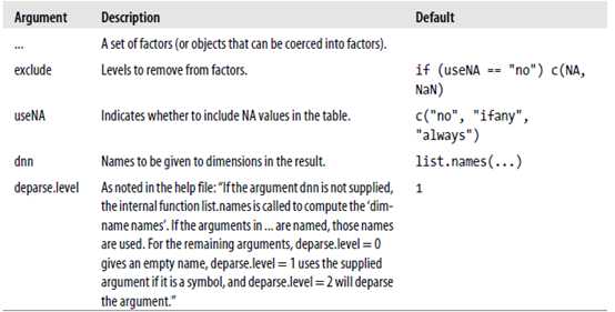
2)一个相关的函数(对于分类值)是table函数。
table(..., exclude = if (useNA == "no") c(NA, NaN), useNA = c("no",
"ifany", "always"), dnn = list.names(...), deparse.level = 1)
The table function returns a table object showing the number of observations that have each possible categorical value。下面是参数说明
?
######例如,we wanted to count the number of left-handed batters,right-handed batters, and switch hitters in 2008。
> table(batting.2008$bats)
?
B L R
118 401 865
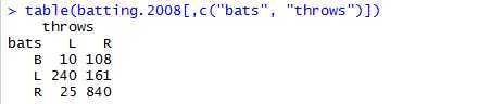
#####又例如,生成一个二维表,显示the number of players who batted and threw with each hand。
3)另一个有用的函数时xtabs函数,which creates contingency tables from factors using
Formulas。
xtabs(formula = ~., data = parent.frame(), subset, na.action,
exclude = c(NA, NaN), drop.unused.levels = FALSE)
注:xtabs函数和table函数类似,区别在于,xtabs允许通过指定一个公式和数据框指定分组(grouping)。例如:use xtabs to tabulate batting statistics by batting arm and league
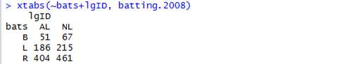
xtabs(~bats+lgID, batting.2008)
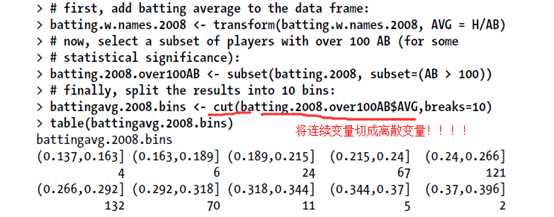
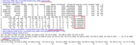
Table函数仅仅对因子变量有效,但是有时候我们也许想要使用数值变量计算tables(列联表)。例如,suppose you wanted to count the number of players with batting averages in certain ranges!此时,可以使用cut函数和table函数
> # first, add batting average to the data frame: > batting.w.names.2008 <- transform(batting.w.names.2008, AVG = H/AB) > # now, select a subset of players with over 100 AB (for some > # statistical significance): > batting.2008.over100AB <- subset(batting.2008, subset=(AB > 100)) > # finally, split the results into 10 bins: > battingavg.2008.bins <- cut(batting.2008.over100AB$AVG,breaks=10) > table(battingavg.2008.bins)
|
?
###对矩阵:下面给出一个例子!
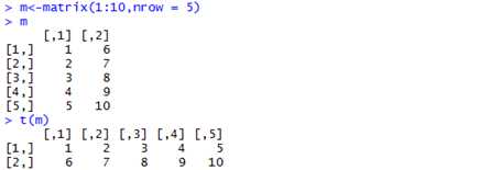
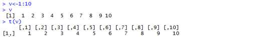
###对向量:当调用一个向量时,向量被当成一个矩阵的单列,因此t函数返回的将是单行矩阵!
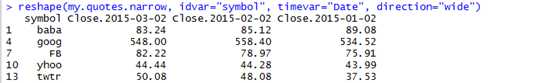
R包含了几个函数,可用于在narrow和wide格式数据间转换。这里使用stock 数据来看看这些函数的用法。
>my.quotes<-get.multiple.quotes(my.tickers,from=as.Date("2015-01-01"),to=as.Date("2015-03-31"), interval="m")
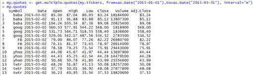
> my.quotes.narrow<-my.quotes[,c(1,2,6)]
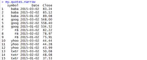
> unstack(my.quotes.narrow, form=Close~symbol) # form是公式,左边表示values,右边表示grouping variables
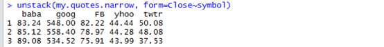
Notice that the unstack operation retains the order of observations but loses the Date column. (It‘s probably best to use unstack with data in which there are only two variables that matter.
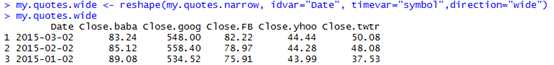
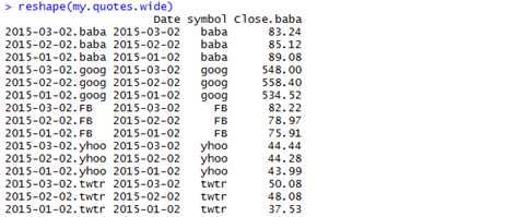
R包含了一个更加强有力的工具,用来改变一个数据框的形状:reshape函数!
在正式讲解如何使用该函数前,先来看几个例子
>my.quotes.wide<-reshape(my.quotes.narrow, idvar="Date", timevar="symbol",direction="wide")
> my.quotes.wide
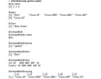
Reshape函数的参数被存储成已创建数据框的属性
另外,还可以让每一行代表一只股票,每一列代表不同的日期
> reshape(my.quotes.narrow, idvar="symbol", timevar="Date", direction="wide")
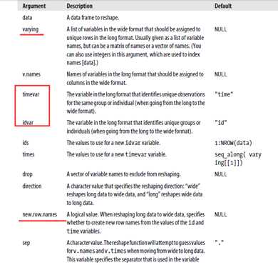
The tricky thing about reshape is that it is actually two functions in one: a function that transforms long data to wide data and a function that transforms wide data to long data. The direction argument specifies whether you want a data frame that is "long" or "wide."
When transforming to wide data, you need to specify the idvar and timevar arguments.When transforming to long data, you need to specify the varying argument.
By the way, calls to reshape are reversible. If you have an object d that was created by a call to reshape, you can call reshape(d) to get back the original data frame:
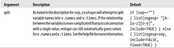
reshape(data, varying = , v.names = , timevar = , idvar = , ids = , times = ,
drop = , direction, new.row.names = , sep = , split = )
下面是参数说明
Many R users (like me) find the built-in functions for reshaping data (like stack,unstack, and reshape) confusing. Luckily, there‘s an alternative.幸运的是,Hadley Wickham这个人开发了一个reshape包(Don‘t confuse the reshape library with the reshape function)
Melting 和 casting
the process of turning a table of data into a set of transactions:melting, and the process of turning the list of transactions into a table:casting!
Reshape使用的例子
首先,来melt股价数据(quote data)
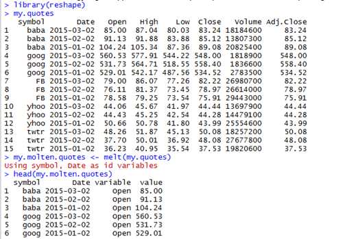
my.molten.quotes <- melt(my.quotes)
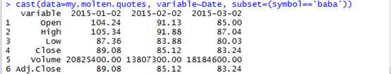
现在,我们有了molten形式的数据,用cast函数进行操作
cast(data=my.molten.quotes, variable~Date, subset=(symbol==‘baba‘))
上面简要的介绍了一下,下面进行详细剖析!
Melt
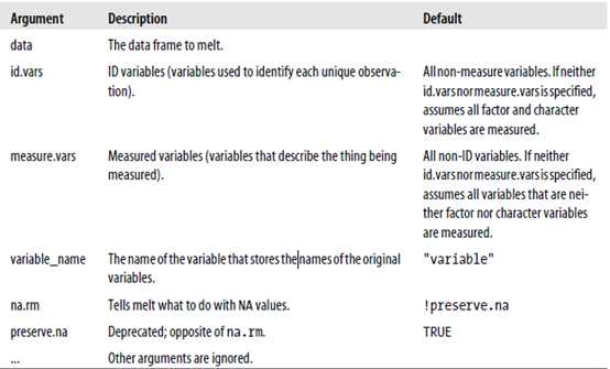
melt is a generic function; the reshape package includes methods for data frames, arrays, and lists。
melt.data.frame(data, id.vars, measure.vars, variable_name, na.rm,
preserve.na, ...)
参数说明
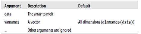
You simply need to specify the dimensions to keep, and melt will melt the array.
melt.array(data, varnames, ...)
the list form of melt will recursively melt each element in the list, join the results, and return the joined form。
melt.list(data, ..., level)
Cast
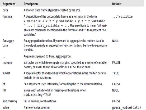
After you have melted your data, you use cast to reshape the results. Here is a description of the arguments to cast
cast(data, formula, fun.aggregate=NULL, ..., margins, subset, df, fill,
add.missing, value = guess_value(data))
Data cleaning doesn‘t mean changing the meaning of data. It means identifying problems caused by data collection, processing, and storage processes and modifying the data so that these problems don‘t interfere with analysis。
?
Data sources often contain duplicate values. Depending on how you plan to use the data, the duplicates might cause problems. It‘s a good idea to check for duplicates in your data
R提供了多种检测重复值的有用工具!
This function returns a logical vector showing which elements are duplicates of values with lower indices
> duplicated(my.quotes.2)
[1] FALSE FALSE FALSE FALSE FALSE FALSE FALSE FALSE FALSE FALSE FALSE
[12] FALSE FALSE FALSE FALSE TRUE TRUE TRUE
检测出来是最后三行重复啦,紧接着去重
> my.quotes.unique <- my.quotes.2[!duplicated(my.quotes.2),]
另外,可以使用unique函数去重,直接完成上述步骤
> my.quotes.unique <- unique(my.quotes.2)
最后还有两个操作函数,你可能觉得在数据分析时非常有用:sorting和ranking函数!
To sort the elements of an object, use the sort function
> w <- c(5, 4, 7, 2, 7, 1)
> sort(w)
[1] 1 2 4 5 7 7
Add the decreasing=TRUE option to sort in reverse order:
> sort(w, decreasing=TRUE)
[1] 7 7 5 4 2 1
还可以设置na.last参数来控制如何处理NA值!
> length(w)
[1] 6
> length(w) <- 7
> # note that by default, NA.last=NA and NA values are not shown
> sort(w)
[1] 1 2 4 5 7 7
> # set NA.last=TRUE to put NA values last
> sort(w, na.last=TRUE)
[1] 1 2 4 5 7 7 NA
> # set NA.last=FALSE to put NA values first
> sort(w, na.last=FALSE)
[1] NA 1 2 4 5 7 7
2)对于数据框的sorting函数使用
To sort a data frame, you need to create a permutation of the indices from the data frame and use these to fetch the rows of the data frame in the correct order. You can generate an appropriate permutation of the indices using the order function:
order(..., na.last = , decreasing = )
#####例子一:
先看order是如何运作的,First, we‘ll define a vector with two elements out of order:
> v <- c(11, 12, 13, 15, 14)
You can see that the first three elements (11, 12, 13) are in order, and the last two (15, 14) are reversed。
> order(v)
[1] 1 2 3 5 4

> v[order(v)]
[1] 11 12 13 14 15
Suppose that we created the following data frame from the vector v and a second vector u:
> u <- c("pig", "cow", "duck", "horse", "rat")
> w <- data.frame(v, u)
> w
v u
1 11 pig
2 12 cow
3 13 duck
4 15 horse
5 14 rat
We could sort the data frame w by v using the following expression
> w[order(w$v),]
v u
1 11 pig
2 12 cow
3 13 duck
5 14 rat
4 15 horse
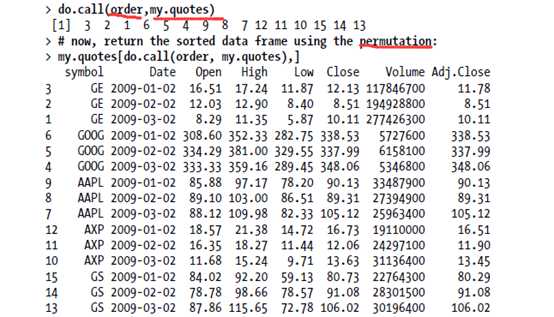
######例子二:按照收盘价来对my.quotes数据框排序
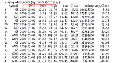
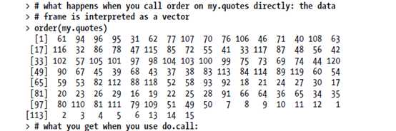
对整个数据框排序有一点不同,
Sorting a whole data frame is a little strange. You can create a suitable permutation using the order function, but you need to call order using do.call for it to work properly. (The reason for this is that order expects a list of vectors and interprets the data frame as a single vector, not as a list of vectors.)
This part of the book explains how to plot data with R.
在R中,绘图的方式有很多种,这里我们只关注三个最流行的包:graphics、lattice和ggplot2!
The graphics package contains a wide variety of functions for plotting data. It is easy to customize or modify charts with the graphics package, or to interact with plots on the screen. The lattice package contains an alternative set of functions for plotting data. Lattice graphics are well suited for splitting data by a conditioning variable. Finally, ggplot2 uses a different metaphor for graphics, allowing you to easily and quickly create stunning charts.
?
?
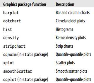
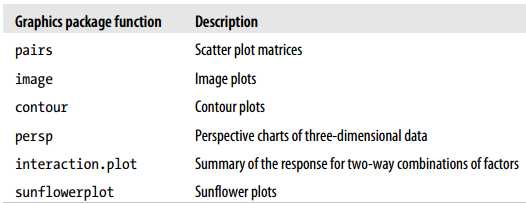
Graphics可以绘制常用的图形类型:bar charts, pie charts, line charts, and scatter plots;还可以绘制不那么常用(less-familiar)的图形:quantile-quantile (Q-Q) plots, mosaic plots, and contour plots。下面的图表显示了graphics包中的图形类型及描述!
可以将R图形显示在屏幕上,也可以保存成多种不同的格式!
绘制散点图的示例数据来自:2008年的癌症案例,2006年按州(state)的toxic废物排放.
> library(nutshell)
> data(toxins.and.cancer)
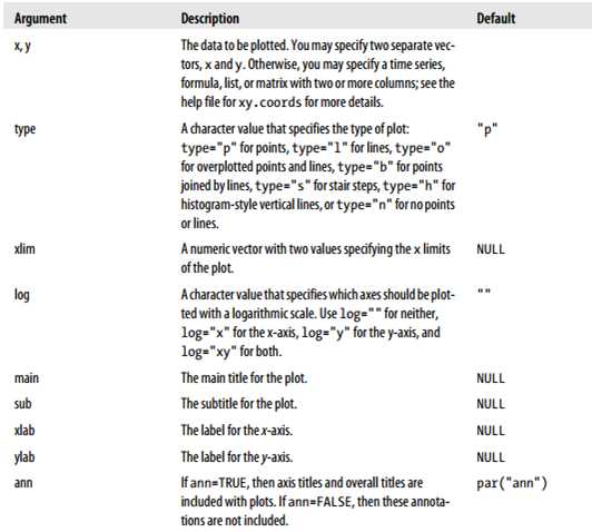
绘制散点图,使用plot函数。plot是一个泛函,plot可以绘制许多不同类型的对象,包括向量、表、时间序列。对于用两个向量绘制简单的散点图,使用plot.default函数:
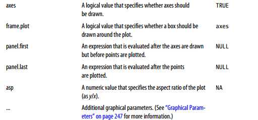
plot(x, y = NULL, type = "p", xlim = NULL, ylim = NULL,
log = "", main = NULL, sub = NULL, xlab = NULL, ylab = NULL,
ann = par("ann"), axes = TRUE, frame.plot = axes,
panel.first = NULL, panel.last = NULL, asp = NA, ...)
@@@@对Plot函数参数的简要描述:
1)第一幅图!比较整体患癌症比例(癌症死亡数除以州人数)与毒素排放量(总体化学毒素排放除以州面积)
> library(nutshell)
> data(toxins.and.cancer)
> head(toxins.and.cancer)
> plot(total_toxic_chemicals/Surface_Area,deaths_total/Population)
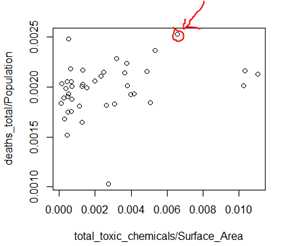
可知, 通过空气传递的毒素和肺癌成强的正相关!
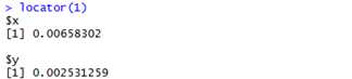
2)假设,你想知道哪一个州和哪一个点相关联。R提供了识别图中点的一些交互工具。可以使用locator函数告诉一个特定点(一组点)的坐标。为了完成这个任务,首先,绘制数据。接下来,输入locator(1).。然后,在打开的图形窗口上点击一点。比如,假设上面绘制的数据,type locator(1),然后,点击右上角高亮的点。你将会在R控制台上看到如下输出结果:
3)另一个识别点的有用函数是identity函数。该函数可以被用于在一副图上交互的标记(label)点。To use identify with the data above:
> plot(air_on_site/Surface_Area, deaths_lung/Population)
> identify(air_on_site/Surface_Area, deaths_lung/Population,labels = State_Abbrev)
[1] 10 12 14 17 22
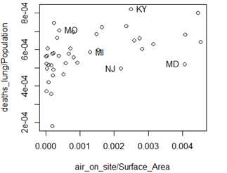
While this command is running, you can click on individual points on the chart,and R will label those points with state names!
> plot(air_on_site/Surface_Area, deaths_lung/Population,xlab=‘Air Release Rate of Toxic Chemicals‘,ylab=‘Lung Cancer Death Rate‘)
> text(air_on_site/Surface_Area, deaths_lung/Population,labels=State_Abbrev,cex=0.5,adj=c(0,-1)) #adj调整位置, cex调整大小!
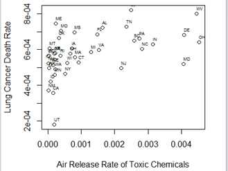
注意到我们使用了xlab、ylab参数向图中添加了x和y轴的标签,使得图形外观更加好看!Text函数对每一个点附近绘制一个标签(我们使用了cex和adj参数对标签的大小和位置进行了微调(tweak) !
那么这个关系统计上显著吗?(see "Correlation tests" on page 384))我们并没有足够的信息来证明这里存在一个因果关系。
5)如果想要绘制数据中的两列到一副图中,plot函数是一个很好的选择。然后,如果要绘制数据中的多列,或者将分裂成不同的类别。或者说,想要绘制一个矩阵的所有列与另一个矩阵的所有列。To plot multiple sets of columns against one another,使用matplot函数:
matplot(x, y, type = "p", lty = 1:5, lwd = 1, pch = NULL,
col = 1:6, cex = NULL, bg = NA,
xlab = NULL, ylab = NULL, xlim = NULL, ylim = NULL,
..., add = FALSE, verbose = getOption("verbose"))
Matplot接收以下参数:
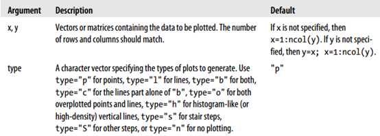
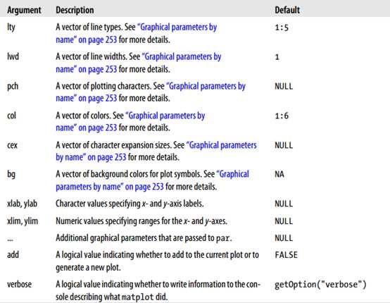
Matplot函数的许多参数和par标准参数名称相同!然而,matplot函数同时生产多幅图,当调用matplot函数时,这些参数以多值向量被指定!
6)如果想要绘制大量的点,可以使用smoothScatter函数。
smoothScatter(x, y = NULL, nbin = 128, bandwidth,
colramp = colorRampPalette(c("white", blues9)),
nrpoints = 100, pch = ".", cex = 1, col = "black",
transformation = function(x) x^.25,
postPlotHook = box,
xlab = NULL, ylab = NULL, xlim, ylim,
xaxs = par("xaxs"), yaxs = par("yaxs"), ...)
> library(nutshell)
> data(batting.2008)
> pairs(batting.2008[batting.2008$AB>100,c(‘H‘,‘R‘,‘SO‘,‘BB‘,‘HR‘)])
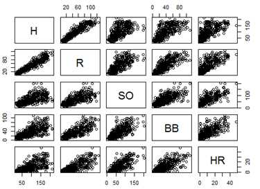
R包含了绘制时间序列数据的工具,plot函数有一个方法:
plot(x, y = NULL, plot.type = c("multiple", "single"),
xy.labels, xy.lines, panel = lines, nc, yax.flip = FALSE,
mar.multi = c(0, 5.1, 0, if(yax.flip) 5.1 else 2.1),
oma.multi = c(6, 0, 5, 0), axes = TRUE, ...)
参数x和y指定ts对象,panel指定如何绘制时间序列(默认是,lines),其他参数指定如何将时间序列break成不同的图形。
1)例如,下面来绘制turkey价格数据!
> library(nutshell)
> data(turkey.price.ts)
> turkey.price.ts
Jan Feb Mar Apr May Jun Jul Aug Sep Oct Nov Dec
2001 1.58 1.75 1.63 1.45 1.56 2.07 1.81 1.74 1.54 1.45 0.57 1.15
2002 1.50 1.66 1.34 1.67 1.81 1.60 1.70 1.87 1.47 1.59 0.74 0.82
2003 1.43 1.77 1.47 1.38 1.66 1.66 1.61 1.74 1.62 1.39 0.70 1.07
2004 1.48 1.48 1.50 1.27 1.56 1.61 1.55 1.69 1.49 1.32 0.53 1.03
2005 1.62 1.63 1.40 1.73 1.73 1.80 1.92 1.77 1.71 1.53 0.67 1.09
2006 1.71 1.90 1.68 1.46 1.86 1.85 1.88 1.86 1.62 1.45 0.67 1.18
2007 1.68 1.74 1.70 1.49 1.81 1.96 1.97 1.91 1.89 1.65 0.70 1.17
2008 1.76 1.78 1.53 1.90
> plot(turkey.price.ts)
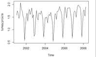
从上图中可以看出,Turkey价格季节性很强(seasonal)。在11月和12月销量(感恩节和万圣节)很大!!!春季销量很少(可能是Easter!)
> acf(turkey.price.ts)
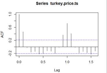
可以看到, points are correlated over 12-month cycles (and inversely correlated over 6-month cycles。
> pacf(turkey.price.ts)
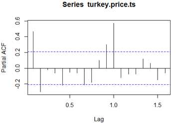
画条形图(列图),使用barplot函数
####构造数据
doctorates <- data.frame (
year=c(2001, 2002, 2003, 2004, 2005, 2006),
engineering=c(5323, 5511, 5079, 5280, 5777, 6425),
science=c(20643, 20017, 19529, 20001, 20498, 21564),
education=c(6436, 6349, 6503, 6643, 6635, 6226),
health=c(1591, 1541, 1654, 1633, 1720, 1785),
humanities=c(5213, 5178, 5051, 5020, 5013, 4949),
other=c(2159, 2141, 2209, 2180, 2480, 2436))
> doctorates
year engineering science education health humanities other
1 2001 5323 20643 6436 1591 5213 2159
2 2002 5511 20017 6349 1541 5178 2141
3 2003 5079 19529 6503 1654 5051 2209
4 2004 5280 20001 6643 1633 5020 2180
5 2005 5777 20498 6635 1720 5013 2480
6 2006 6425 21564 6226 1785 4949 2436
注:上面的数据在nutshell包中也有,可以直接data加载!
####转化成矩阵,便于绘图!(make this into a matrix!)
> doctorates.m<-as.matrix(doctorates[2:7])
> rownames(doctorates.m)<-doctorates[,1]
> doctorates.m
engineering science education health humanities other
2001 5323 20643 6436 1591 5213 2159
2002 5511 20017 6349 1541 5178 2141
2003 5079 19529 6503 1654 5051 2209
2004 5280 20001 6643 1633 5020 2180
2005 5777 20498 6635 1720 5013 2480
2006 6425 21564 6226 1785 4949 2436
由于barplot函数不能处理数据框,因此,这里我们创建了一个矩阵对象!
1.1)首先来看看2001年博士学位授予条状图(第一行数据!!!)
> barplot(doctorates.m[1,])
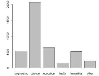
可以看到,R默认显示了 y-axis along with the size of each bar,但是未显示x-axis轴。R会自动使用列名来对每一个bars命名。
1.2)Suppose that we wanted to show all the different years as bars stacked next to one another. Suppose that we also wanted the bars plotted horizontally and wanted to show a legend for the different years。
> barplot(doctorates.m, beside=TRUE, horiz=TRUE, legend=TRUE, cex.names=.75)
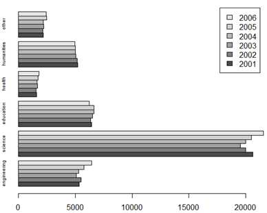
1.3)最后, suppose that we wanted to show doctorates by year as stacked bars()。这里我们需要对矩阵进行转化,每一列是年,每一行是一个discipline(学科)。同时,还需要确保足够的空间来显示legend,这里对y-axis的limits进行了扩展!
> barplot(t(doctorates.m), legend=TRUE, ylim=c(0, 66000))
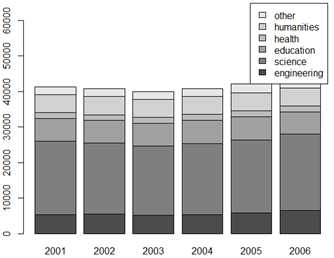
下面是对barplot函数的详细描述!
barplot(height, width = 1, space = NULL,
names.arg = NULL, legend.text = NULL, beside = FALSE,
horiz = FALSE, density = NULL, angle = 45,
col = NULL, border = par("fg"),
main = NULL, sub = NULL, xlab = NULL, ylab = NULL,
xlim = NULL, ylim = NULL, xpd = TRUE, log = "",
axes = TRUE, axisnames = TRUE,
cex.axis = par("cex.axis"), cex.names = par("cex.axis"),
inside = TRUE, plot = TRUE, axis.lty = 0, offset = 0,
add = FALSE, args.legend = NULL, ...)
Barplot函数非常灵活,其参数描述如下:
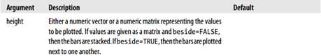
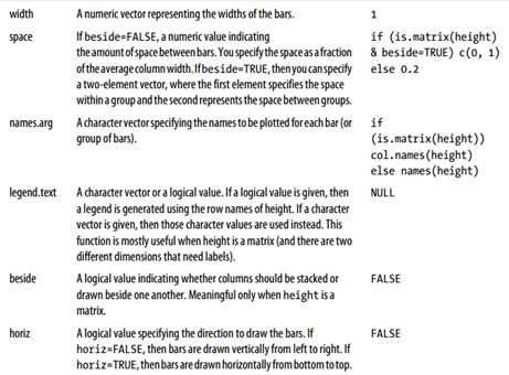
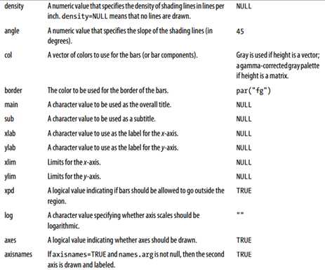
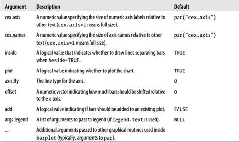
One of the most popular ways to plot data is the pie chart. Pie charts can be an effective way to compare different parts of a quantity, though there are lots of good reasons not to use pie charts
下面是pie函数:
pie(x, labels = names(x), edges = 200, radius = 0.8,
clockwise = FALSE, init.angle = if(clockwise) 90 else 0,
density = NULL, angle = 45, col = NULL, border = NULL,
lty = NULL, main = NULL, ...)
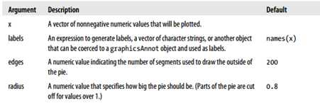
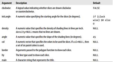
> domestic.catch.2006 <- c(7752, 1166, 463, 108)
> names(domestic.catch.2006) <- c("Fresh and frozen", "Reduced to meal, oil, etc.","Canned", "Cured")
> pie(domestic.catch.2006, init.angle=100, cex=.6)
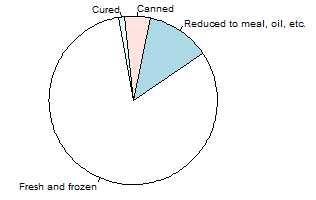
# note: cex.6 setting shrinks text size by 40% so you can see the labels
The graphics package includes some very useful, and possibly unfamiliar, tools for looking at categorical data。
1)假设我们依据一个数值查看一组分类/类别的条件密度。使用cdplot函数!
cdplot(x, y,
plot = TRUE, tol.ylab = 0.05, ylevels = NULL,
bw = "nrd0", n = 512, from = NULL, to = NULL,
col = NULL, border = 1, main = "", xlab = NULL, ylab = NULL,
yaxlabels = NULL, xlim = NULL, ylim = c(0, 1), ...)
调用公式时cdplot的形式
cdplot(formula, data = list(),
plot = TRUE, tol.ylab = 0.05, ylevels = NULL,
bw = "nrd0", n = 512, from = NULL, to = NULL,
col = NULL, border = 1, main = "", xlab = NULL, ylab = NULL,
yaxlabels = NULL, xlim = NULL, ylim = c(0, 1), ...,
subset = NULL)
Cdplot函数使用density函数来计算各种数值的核密度估计(kernel density estimates),然后plot these estimates。下面是cdplot的参数列表:
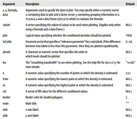
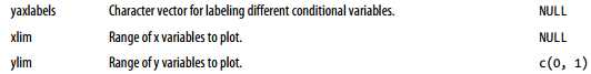

1.1)例子:看看batting hand分布是如何随2008年MLB球员中的平均击球次数(batting average)变化的。
> batting.w.names.2008 <- transform(batting.2008,AVG=H/AB, bats=as.factor(bats), throws=as.factor(throws))
> head(batting.w.names.2008)
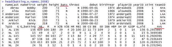
> cdplot(bats~AVG,data=batting.w.names.2008,subset=(batting.w.names.2008$AB>100))
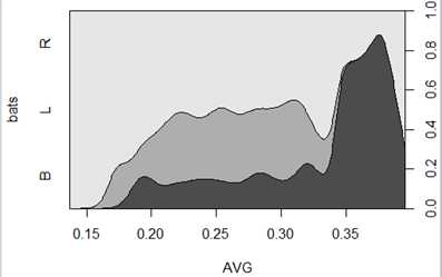
As you can see, the proportion of switch hitters (bats=="B") increases with higher batting average
2)假设仅仅想针对不同的分类变量绘制观测值的比例。可视化这类数据的工具很多,R中最有意思的一个函数是mosaicplot( showing the number of observations with certain properties)。一副mosaic plot(马赛克图/拼花图)显示了对应于不同因子值的一组盒子(boxes)。The x-axis corresponds to one factor and the y-axis to another factor。使用mosaicplot函数来创建马赛克图,下面是针对一个列联表(contingency table)的mosaicplot函数:
mosaicplot(x, main = deparse(substitute(x)),
sub = NULL, xlab = NULL, ylab = NULL,
sort = NULL, off = NULL, dir = NULL,
color = NULL, shade = FALSE, margin = NULL,
cex.axis = 0.66, las = par("las"),
type = c("pearson", "deviance", "FT"), ...)
还有另一种是允许将数据指定为一个公式或数据框的形式!
mosaicplot(formula, data = NULL, ...,
main = deparse(substitute(data)), subset,
na.action = stats::na.omit)
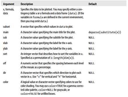
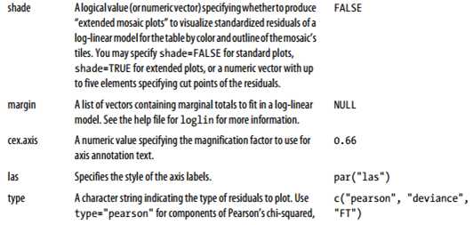
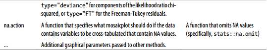
2.1)例子:创建一个显示2008年MLB击球手(batters)数量的马赛克图。
On the x-axis, we‘ll show batting hand (left, right, or both), and on the yaxis we‘ll show throwing hand (left or right).该函数可以接收一个矩阵、公式和数据框。在本例中,我们使用公式和数据框:
> mosaicplot(formula=bats~throws, data=batting.w.names.2008, color=TRUE) #bats和throws都是分类变量!
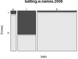
3.1)例子:数据和马赛克图的数据一样,下面使用splineplot函数来绘制一个样条图
> spineplot(formula=bats~throws, data=batting.w.names.2008)
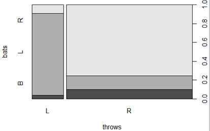
4)Another function for looking at tables of data is assocplot函数。绘制出来的图被称为
Cohen-Friendly association图形。(This function plots a set of bar charts, showing the deviation of each combination of factors from independence)
4.1)例子:数据沿用上一个例子的数据
> assocplot(table(batting.w.names.2008$bats, batting.w.names.2008$throws),
xlab="Throws", ylab="Bats")
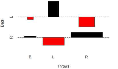
R包括了一些对三维数据可视化的函数。所有这些函数都能被用于绘制矩阵值。(Row indices correspond to x values,column indices to y values, and values in the matrix to z values)
persp(x = seq(0, 1, length.out = nrow(z)),
y = seq(0, 1, length.out = ncol(z)),
z, xlim = range(x), ylim = range(y),
zlim = range(z, na.rm = TRUE),
xlab = NULL, ylab = NULL, zlab = NULL,
main = NULL, sub = NULL,
theta = 0, phi = 15, r = sqrt(3), d = 1,
scale = TRUE, expand = 1,
col = "white", border = NULL, ltheta = -135, lphi = 0,
shade = NA, box = TRUE, axes = TRUE, nticks = 5,
ticktype = "simple", ...)
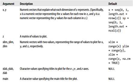
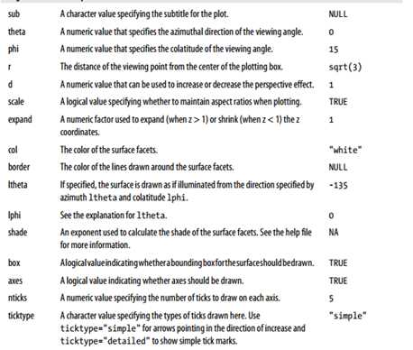
1.1)例子:使用Yosemite Valley的三维数据。
Specifically, let‘s look toward Half Dome. To plot this elevation data(海拔数据), I needed to make two transformations. First, I needed to flip(掷/快速翻动) the data horizontally. In the data file, values move east to west (or left to right) as x indices increase and from north to south (or top to bottom) as y indices increase. Unfortunately, persp plots y coordinates slightly differently. Persp plots increasing y coordinates from bottom to top. So I selected y indices in reverse order。
# load the data:
> library(nutshell)
> data(yosemite)
> head(yosemite)

# check dimensions of data
> dim(yosemite)
[1] 562 253
> yosemite.flipped<-yosemite[,seq(from = 253,to=1)]
> head(yosemite.flipped)
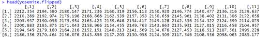
下一步,仅仅选择海拔点(elevation points)的方形子集(square subset)。这里,我们仅仅Yosemite矩阵最右边(rightmost)的253列!(Note the "+ 1" in this statement; that‘s to make sure that we take exactly 253 columns. (This is to avoid a fencepost error.)
To plot the figure, I rotated the image by 225° (through theta=225) and changed the viewing angle to 20° (phi=20). I adjusted the light source to be from a 45° angle (ltheta=45) and set the shading factor to 0.75 (shade=.75) to exaggerate topological features. Putting it all together。
> # create halfdome subset in one expression:
# 选择310:562行,253:1列的方形数据!
> halfdome <- yosemite[(nrow(yosemite) - ncol(yosemite) + 1):562,seq(from=253,to=1)]
> persp(halfdome,col=grey(.25), border=NA, expand=.15,theta=225, phi=20, ltheta=45, lphi=20, shade=.75)
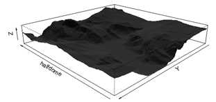
image(x, y, z, zlim, xlim, ylim, col = heat.colors(12),
add = FALSE, xaxs = "i", yaxs = "i", xlab, ylab,
breaks, oldstyle = FALSE, ...)
下面是image函数的参数说明
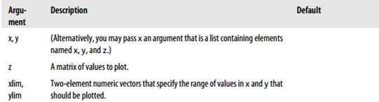
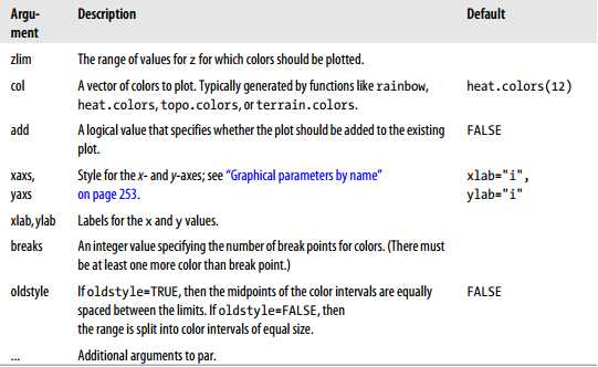
下面是基于Yosemite Valley数据生成的image图表达式:
> data(yosemite)
> image(yosemite, asp=253/562, ylim=c(1,0), col=sapply((0:32)/32, gray))
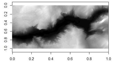
heatmap(x, Rowv=NULL, Colv=if(symm)"Rowv" else NULL,
distfun = dist, hclustfun = hclust,
reorderfun = function(d,w) reorder(d,w),
add.expr, symm = FALSE, revC = identical(Colv, "Rowv"),
scale=c("row", "column", "none"), na.rm = TRUE,
margins = c(5, 5), ColSideColors, RowSideColors,
cexRow = 0.2 + 1/log10(nr), cexCol = 0.2 + 1/log10(nc),
labRow = NULL, labCol = NULL, main = NULL,
xlab = NULL, ylab = NULL,
keep.dendro = FALSE, verbose = getOption("verbose"), ...)
4)此外,还有contour函数。
contour(x = seq(0, 1, length.out = nrow(z)),
y = seq(0, 1, length.out = ncol(z)),
z,
nlevels = 10, levels = pretty(zlim, nlevels),
labels = NULL,
xlim = range(x, finite = TRUE),
ylim = range(y, finite = TRUE),
zlim = range(z, finite = TRUE),
labcex = 0.6, drawlabels = TRUE, method = "flattest",
vfont, axes = TRUE, frame.plot = axes,
col = par("fg"), lty = par("lty"), lwd = par("lwd"),
add = FALSE, ...)
下面是contour函数的参数列表:
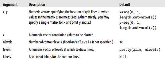
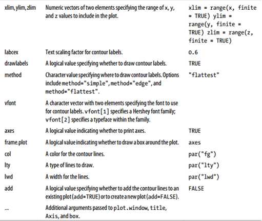
4.1)例子:使用Yosemite Valley数据绘制一个contour图形的表达式
> contour(yosemite, asp=253/562, ylim=c(1, 0))
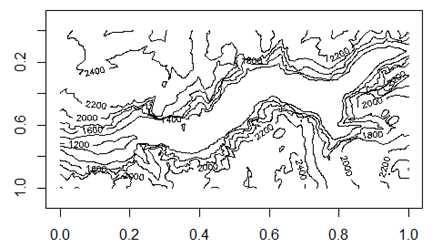
As with image, we needed to flip the y-axis and to specify an aspect ratio!
当进行数据分析时,理解一份数据的分布是很重要的。它可以告诉你是否数据中存在奇异值(outliers),是否某一个建模技术对数据合适等等。
1.1)例子:先来看看在2008年MLB赛季击球手(batters)的plate appearances的数量。
# 加载数据集
> library(nutshell)
> data(batting.2008)
# Let‘s calculate the plate appearances for each player and then plot a histogram
#注意:PA (plate appearances) = AB (at bats) + BB (base on balls) + HBP (hit by pitch) + SF (sacrifice flies) + SH (sacrifice bunts)
> batting.2008 <- transform(batting.2008,PA=AB+BB+HBP+SF+SH)
> hist(batting.2008$PA)
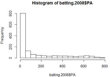
The histogram shows that there were a large number of players with fewer than 50 plate appearances. If you were to perform further analysis on this data (for example, looking at the average on-base percentage [OBP]), you might want to exclude these players from your analysis.
1.2)生成第二幅直方图,this time excluding players with fewer than 25 at bats. We‘ll also increase the number of bars, using the breaks argument to specify that we want 50 bins!
> hist(batting.2008[batting.2008$PA>25, "PA"], breaks=50, cex.main=.8)
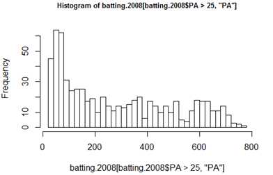
> plot(density(batting.2008[batting.2008$PA>25, "PA"]),cex.main = 0.9)
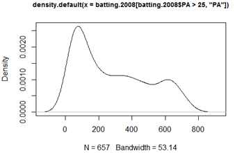
关于density函数的一个简要例子说明
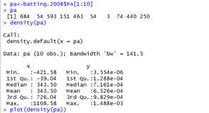
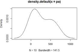
Density返回的对象中包括:x,y,bw,n,call,data.name,has.na!
X和y是根据核函数估计出来的连续取值,用来生成平滑曲线的!
另外,对于核密度图的一个常用tricks(addition)是使用rug函数。
#### add a rug to the kernel density plot with an expression like:
> rug(batting.2008[batting.2008$PA>25, "PA"])
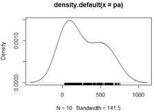
在R中使用qqnorm函数生成这类图,Without arguments, this function will plot the distribution of points in each quantile, assuming a theoretical normal distribution!
> qqnorm(y = batting.2008$AB)
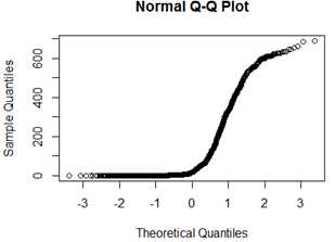
If you would like to compare two actual distributions, or compare the data distribution to a different theoretical distribution, then try the function qqplot.
另一个可视化分布的有用方式是box plot.
临近值(adjacent values)用来显示极值(extreme values!),但是不总是适用于绝对最大值或最小值。当有远离四分位间距之外的值时,这些异常值(outlying values)会被单独绘制出来。具体说,临近值是如何被计算出来的呢?上部临近值=小于或等于上部四分位值的最大观测值+1.5倍四分位间距的长度。超出whiskers范围的值被称为outside values,被单独绘制!
绘制box plot,使用的是boxplot函数。
###下面是针对向量的boxplot函数的默认方法:
boxplot(x, ..., range = 1.5, width = NULL, varwidth = FALSE,
notch = FALSE, outline = TRUE, names, plot = TRUE,
border = par("fg"), col = NULL, log = "",
pars = list(boxwex = 0.8, staplewex = 0.5, outwex = 0.5),
horizontal = FALSE, add = FALSE, at = NULL)
###下面是指定formula形式的boxplot函数:
boxplot(formula, data = NULL, ..., subset, na.action = NULL)
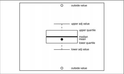
下面是参数说明:
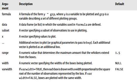
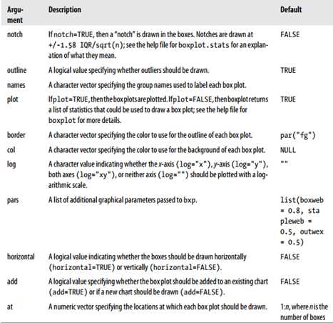
> batting.2008 <- transform(batting.2008,OBP=(H+BB+HBP)/(AB+BB+HBP+SF))
> boxplot(OBP~teamID,data=batting.2008[batting.2008$PA>100 & batting.2008$lgID=="AL",],cex.axis=.7)
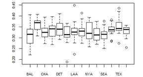
R中的图表(graphics)是被画在一个graphics devices上面的。可以手动指定一个图形设备或者使用默认设置。在一个交互式的R环境中,默认是使用将图形绘制在屏幕上的设备(device)。在window系统上,使用的是windows设备。在大多数Unix系统中,使用的X11。在Mac OS X中,使用的是quartz设备。可以使用bmp、jpeg、png和tiff设备生成普通格式的图形。其他设备(包括postscript、pdf、pictex(生成LaTeX/PicTex)、xfig和bitmap)
大多数设备都允许指定 width,height,输出的point size(参数是width、height和pointsize参数!)。对于生成文件(files)的设备,通常使用file参数名,当将一个图形写入到一个文件中后,记得调用dev.off函数关掉和保存文件!!!
>png("scatter.1.pdf", width=4.3, height=4.3, units="in", res=72)
> attach(toxins.and.cancer)
> plot(total_toxic_chemicals/Surface_Area, deaths_total/Population)
> dev.off()
有很多改变R绘图的方式,最直观(intuitive)的就是通过设置传递给绘图函数(charting function)的参数来达到此目的。另外一种自定义图形的方式是通过设置分区参数(session parameters)。还有一种change a chart的方式就是通过修改图形的函数(比如,添加titles,trend lines等)。最后一种方式就是从头开始写自己的绘图函数(charting function)。
This section describes common arguments and parameters for controlling how charts are plotted.
常用的绘图函数参数简介:
Conveniently, most charting functions in R share some arguments. Here is a table of common arguments for charting functions.
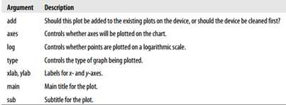
This section describes the graphical parameters available in the graphics package。
In most cases, you can specify these parameters as arguments to graphics functions. However, you can also use the par function to set graphics parameters。Par函数sets the graphics functions for a specific graphics device. These new settings will be the defaults for any new plot until you close the device。
想要设置一次参数,然后连续绘制几幅图形或者多次使用相同的参数设置,设置par函数非常有用。可以写一个设置正确参数的函数,然后每当你想要绘制一些图形的时候就调用它:
> my_graphics_params <- function () {
par(some graphics parameters)
}
用par检查(check)一个参数的值,使用字符串指定值的名称;设置一个参数值,使用参数名(parameter name)作为一个参数名(argument name)。几乎所有的参数都能被读取或重写,唯一的例外就是cin、cra、csi、cxy、din,这些只能被读取;
> par("bg")
[1] "transparent"
You could use the par function to change the bg parameter to "white":
> par(bg="white")
> par("bg")
[1] "white"
Titles和axis labels被称为chart annotation。
> par(ann = FALSE) ; > plot(x = 1:5,y = 21:25)
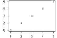
R allows you to control the size of the margin around a plot, The whole graphics device is called the device region. The area where data is plotted is called the plot region。
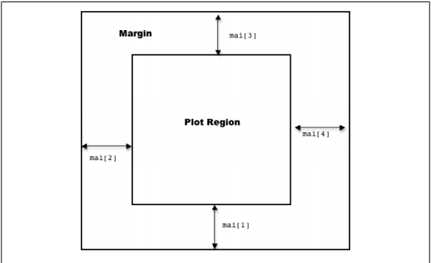

默认下, R maximizes the use of available space out to the margins (pty="m"), but you can easily ask R to use a square region by setting pty="s"!
> par(‘mai‘)
[1] 1.360000 1.093333 1.093333 0.560000
> par(‘mar‘)
[1] 5.1 4.1 4.1 2.1
> par(‘mex‘)
[1] 1
1)在R中,可以在相同的chart area内绘制多幅图,这便是mfcol参数。例如:下面在图形区域绘制六副图(三行两列: in three rows of two columns)
> par(mfcol=c(3, 2))
Each time a new figure is plotted, it will be plotted in a different row or column within the device
从top-left corner开始。每一次添加一幅图,从top到bottom首先fill每一列,然后,移动到右边的下一列(moving to the next column to the right)。
1.1)例子:绘制六福不同的图形
> png("~/Documents/book/current/figs/multiplefigs.1.pdf",
+ width=4.3, height=6.5, units="in", res=72)
> par(mfcol=c(3, 2))
> pie(c(5, 4, 3))
> plot(x=c(1, 2, 3, 4, 5), y=c(1.1, 1.9, 3, 3.9, 6))
> barplot(c(1, 2, 3, 4, 5))
> barplot(c(1, 2, 3, 4, 5), horiz=TRUE)
> pie(c(5, 4, 3, 2, 1))
> plot(c(1, 2, 3, 4, 5, 6), c(4, 3, 6, 2, 1, 1))
> dev.off()
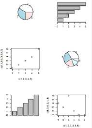
如果在图形设备上绘制子图(subplots)矩阵,可以视同参数mfg=c(row, column, nrows,ncolumns)来指定下一副图的位置!
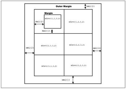
在图形区域的周围有一个outer margin;可以通过参数omi、oma、omd来控制‘在每一副图中,都有一个第二margin area,通过mai、mar、mex控制。如果你自己的图形函数,也许你会使用xpd参数来控制where graphics are clipped!
查看当前图形区域(within the grid)的大小,使用pin参数,获取图形区域的坐标,使用plt参数。查看使用标准化设备坐标(normalized device coordinates)的当前图形区域的dimensions,使用fig参数!
You may find it easier to use the functions layout or split.screen. Better still, use the packages grid or lattice
Many parameters control the way text is shown within a plot!
Text size
参数介绍:
ps:指定默认的文本point size;cex:指定默认的文本scaling factor(即文本大小);cex.axis:针对坐标轴注释;cex.lab针对x和y轴的labels;cex.main:针对主标题;cex.sub针对子标题(subtitles)。
1)确定point size for a chart title, multiply ps*cex*main!
可能还会用到只读的参数:cin,cra,csi和cxy来查看字符的大小!
###Typeface
文本风格通过font参数来指定;You can specify the style for the axis with font.axis, for labels with font.lab, for main titles with font.main, and for subtitles with font.sub.
###Alignment和spacing.
To control how text is aligned, use the adj parameter. To change the spacing between lines of text, use the lheight parameter!
###Rotation
To rotate each character, use the crt parameter. To rotate whole strings,use the srt parameter
@@@首先,取得这些参数的默认值,然后对其进行微调,查看效果!
>unlist(par(‘ps‘,‘cex‘,‘cex.axis‘,‘cex.lab‘,‘cex.main‘,‘cex.sub‘,‘font‘,‘font.axis‘,‘font.lab‘,‘font.main‘,‘font.sub‘,‘adj‘,‘crt‘,‘srt‘) )

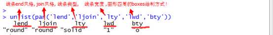

可以使用很多方式来指定颜色。作为一个字符串,使用RGB元素, 或者通过整数索引引用(reference)一个调色板(palette)。获取一个有效的颜色名称列表,使用colors函数。使用RGB组件指定一个颜色, 使用形如"#RRGGBB"格式的字符串, 其中RR,GG,BB是16进制值,用于分别指定红色,绿色,蓝色的量。为了查看或改变一个颜色调色板,使用palette函数。其他函数还有:rgb, hsv, hcl, gray, and rainbow!
#####(1)根据colors()常量(包含有 657中颜色)生成一个颜色带,如下:
idx<-1:657
colorband<-colors()
plot(1,1,xlim = c(1,700),ylim=c(1,700))
j=1
> for(i in idx) {
abline(h=i,col=colorband[j])
j=j+1
}
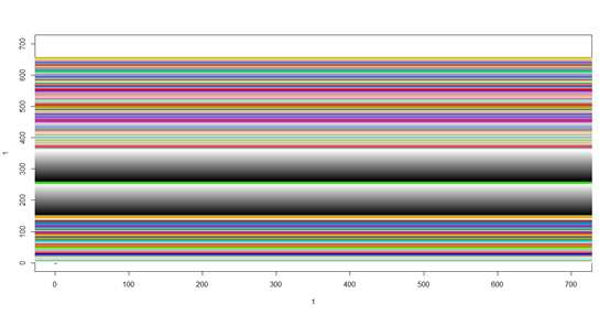
#####(2)根据rainbow()函数生成12中颜色的颜色带
> plot(1,1,xlim = c(1,15),ylim=c(1,15))
> rainbowband<-rainbow(12)
> j=1
> for(i in idx[1:12]) {
abline(h=i,col=rainbowband[j],lwd=4)
j=j+1
}
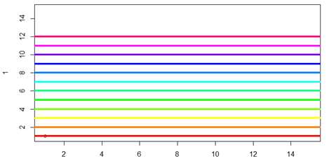
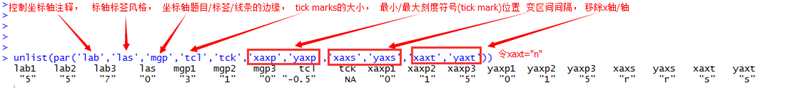
可以通过指定pch参数来改变点的符号,获取点类型列表,使用points函数
下表显示了能够被par()图形参数函数设置的所有R可用图形参数:
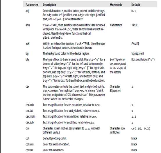
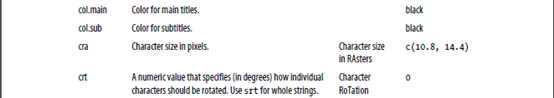
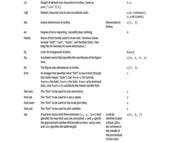
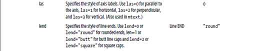
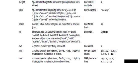
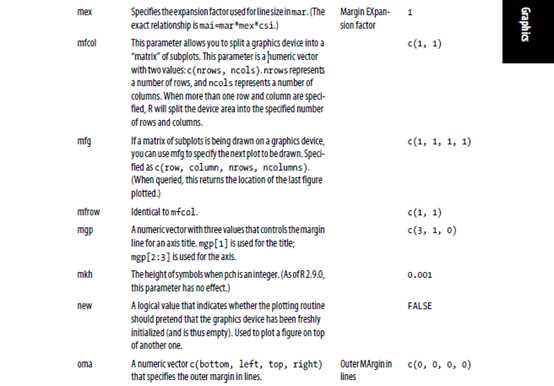
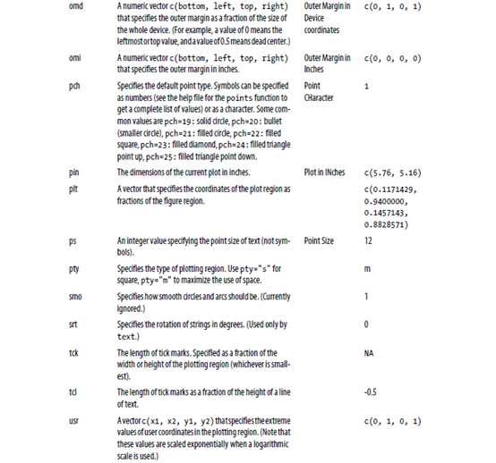
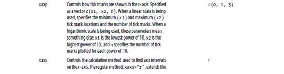
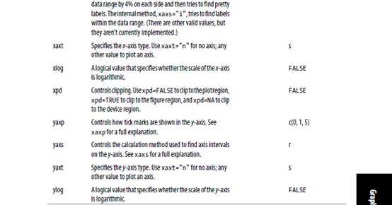
下面是一个被高级图形函数调用对应低级图形函数的图形列表(我们通常可以查看低级函数的参数来确定如何自定义由相应高级函数产生的图形的外观)
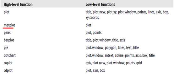
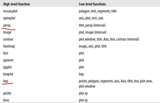
可以使用points函数在一副图上绘制点
points(x, y = NULL, type = "p", ...)
# 这对于向现有图(通常是散点图)中添加额外的点非常的有用,这些额外添加的点一般会用不同的颜色或图形符号。最有用的参数有:col(指定绘制点的前景色),bg(指定点的背景色),pch(指定绘制的字符),cex(指定绘制点的大小),lwd(指定绘制符号的线宽-line width)。
同样,还能使用matpoints函数向现有的矩阵图中添加点:
matpoints(x, y, type = "p", lty = 1:5, lwd = 1, pch = NULL,col = 1:6, ...)
lines(x, y = NULL, type = "l", ...) #
# 和点一样,lines也是被用于添加到一个现有图中。Lines函数在现有图中绘制一组线段(lines segments:x和y的值指定线段间的交点)。一些有用的参数是:lty(线类型-line type),lwd(线宽-line width),col(线颜色-line color),lend(线段结尾处的风格-line end style),ljoin(线相交处的风格-line join style),lmitre(线斜接处的风格-line mitre style)。
同样,可以使用matlines向现有图中添加线:
matlines (x, y, type = "l", lty = 1:5, lwd = 1, pch = NULL,col = 1:6, ..)
在当前图形设备上绘制曲线,使用curve函数
curve(expr, from = NULL, to = NULL, n = 101, add = FALSE,type = "l", ylab = NULL, log = NULL, xlim = NULL, ...)
### 下面是该函数的参数列表:
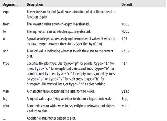
#####举个简答的例子:画正弦/余弦函数
> curve(sin, -2*pi, 2*pi, xname = "t")
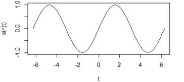
> plot(cos, -pi, 3*pi)
> curve(cos, xlim = c(-pi, 3*pi), n = 1001, col = "blue", add = TRUE) ##使用add参数
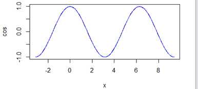
?
?
## 使用text函数向现有图添加文本。
text (x, y = NULL, labels = seq_along(x), adj = NULL,pos = NULL, offset = 0.5, vfont = NULL,
cex = 1, col = NULL, font = NULL, ...)
## 下面是参数列表
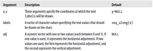
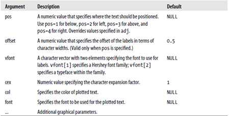
## 在整个图形区域绘制一根线条,使用abline函数:
abline(a = NULL, b = NULL, h = NULL, v = NULL, reg = NULL,coef = NULL, untf = FALSE, ...)
## 下面是abline函数的参数列表:
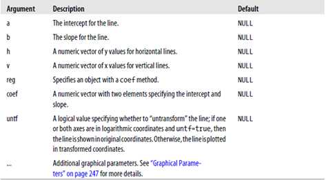
## 一般而言,调用一次abline函数来画一根直线。例如:
@@@(1)draw a simple plot as a background
> plot(x=c(0, 10), y=c(0, 10))
>(2) # plot a horizontal line at y=4
> abline(h=4)
> #(3) plot a vertical line at x=3
> abline(v=3)
> #(4) plot a line with a y-intercept of 1 and slope of 1
> abline(a=1, b=1)
> # (5)plot a line with a y-intercept of 10 and slope of -1,but this time, use the coef argument:
> abline(coef=c(10, -1))
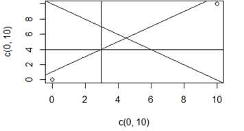
@@@ abline还可以绘制所有指定的线,例如:
> plot(x=c(0, 10), y=c(0, 10))
> # plot a grid of lines between 1 and 10
> abline(h=1:10, v=1:10)
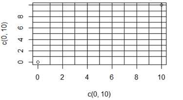
@@@ 补充:如果想要在一副图上绘制一网格,使用grid函数:
grid(nx = NULL, ny = nx, col = "lightgray", lty = "dotted",lwd = par("lwd"), equilogs = TRUE)
## 举个例子吧!
> plot(x=c(0, 10), y=c(0, 10))
> grid(nx = 10,ny = 5,col = rainbow(15),lwd = 3) # 生成一个nx*ny的网格
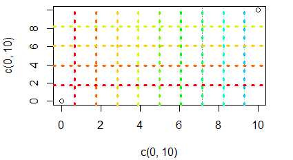
# 向现有图中添加-绘制多边形
polygon(x, y = NULL, density = NULL, angle = 45,border = NULL, col = NA, lty = par("lty"), ..
# x和y参数指定多边形的顶点(vertices)。例如:
> polygon(x=c(2, 2, 4, 4), y=c(2, 4, 4, 2)) # 以(3,3)为中心在图形上绘制一个2*2正方形!
@@@ 特例:如果有些时候,你想画长方形(rectangle),使用rect函数即可!
rect(xleft, ybottom, xright, ytop, density = NULL, angle = 45,col = NA, border = NULL, lty = par("lty"), lwd = par("lwd"),...)
举个例子吧:
> plot(c(100, 250), c(300, 450), type = "n", xlab = "", ylab = "",
+ main = "2 x 11 rectangles; ‘rect(100+i,300+i, 150+i,380+i)‘")
> i <- 4*(0:10) ##指定长方形间的间距 0 4 8 12 16 20 24 28 32 36 40
> ## draw rectangles with bottom left (100, 300)+i
> ## and top right (150, 380)+i
> rect(100+i, 300+i, 150+i, 380+i, col = rainbow(11, start = 0.7, end = 0.1))
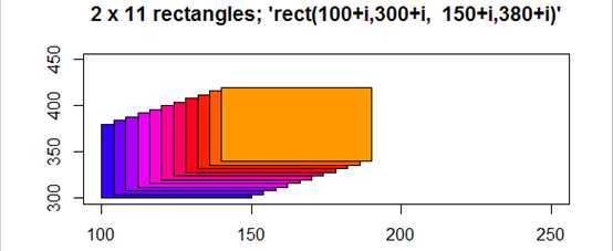
# 画线段/和箭头
segments(x0, y0, x1, y1,col = par("fg"), lty = par("lty"), lwd = par("lwd"),...)
## x0, y0:coordinates of points from which to draw.
## x1, y1:coordinates of points to which to draw
# 该函数根据(x0[i],y0[i]) to (x1[i], y1[i])指定的顶点对绘制一组线段!
# 举个小例子:
> x <- stats::runif(12); y <- stats::rnorm(12)
> i <- order(x, y); x <- x[i]; y <- y[i]
> plot(x, y, main = "arrows(.) and segments(.)")
> i
[1] 10 6 12 9 5 4 7 1 2 3 8 11
> s <- seq(length(x)-1)
> arrows(x[s], y[s], x[s+1], y[s+1], col= 1:3)
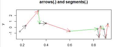
> plot(x, y, main = "arrows(.) and segments(.)")
> segments(x[s], y[s], x[s+2], y[s+2], col= ‘pink‘)
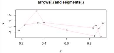
# 向一副图中添加legend(图例)!
legend(x, y = NULL, legend, fill = NULL, col = par("col"),lty, lwd, pch,angle = 45, density = NULL, bty = "o", bg = par("bg"),box.lwd = par("lwd"), box.lty = par("lty"), box.col = par("fg"),pt.bg = NA, cex = 1, pt.cex = cex, pt.lwd = lwd, xjust = 0, yjust = 1, x.intersp = 1, y.intersp = 1,adj = c(0, 0.5), text.width = NULL, text.col = par("col"),merge = do.lines && has.pch, trace = FALSE,plot = TRUE, ncol = 1, horiz = FALSE, title = NULL,inset = 0, xpd, title.col = text.col)
# 下面是参数列表!
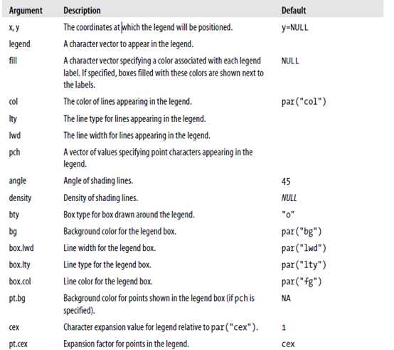
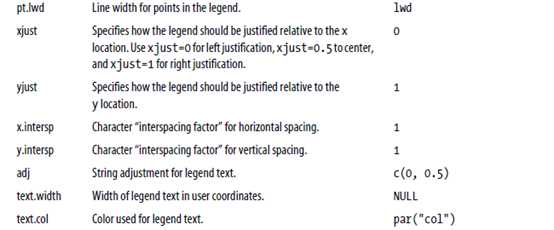
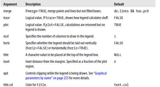
# 添加图形注解
title(main = NULL, sub = NULL, xlab = NULL, ylab = NULL,line = NA, outer = FALSE, ...)
# 该函数可以添加:a main title (main), a subtitle (sub), an x-axis label (xlab), and a y-axis label (ylab);指定line的值来将标签从图形的边缘外移!指定outer=TRUE,即将标签放在外边缘
# 添加坐标轴
axis(side, at = NULL, labels = TRUE, tick = TRUE, line = NA,
pos = NA, outer = FALSE, font = NA, lty = "solid",
lwd = 1, lwd.ticks = lwd, col = NULL, col.ticks = NULL,
hadj = NA, padj = NA, ...)
# 下面是参数列表:
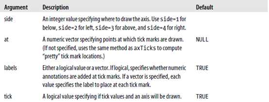
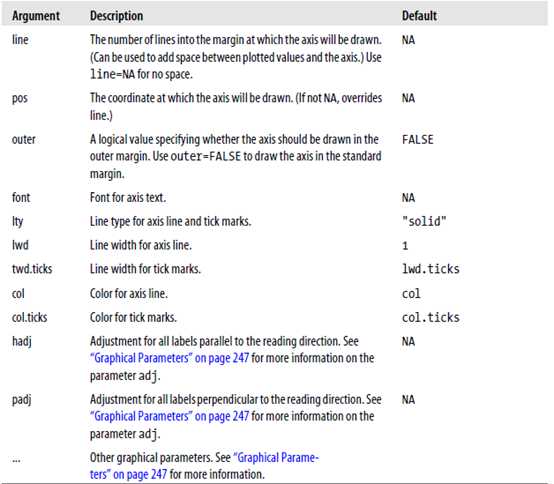
# 用于在当前图形区域绘制一个box。一般当我们在一个图形设备中绘制多幅图时比较有用!
box(which = "plot", lty = "solid", ...)
### which参数指定在哪里绘制box,可取的值有:"plot,""figure," "inner," and "outer")!
# 用于向图形的边缘(margin)添加文本!
mtext(text, side = 3, line = 0, outer = FALSE, at = NA,adj = NA, padj = NA, cex = NA, col = NA, font =NA, ...)
### side参数指定在哪里绘制文本(side = 1 for bottom, side =2 for left, side = 3 for top, and side = 4 for right);line参数指定在哪里写文本(就"margin lines"而言, 从与图形区域最近的0开始);
# 向透视图中添加线或点(透视图使用persp函数绘制)
trans3d(x,y,z, pmat)
# This function takes vectors of points x, y, and z and translates them into the correct screen position. The argument pmat is a perspective matrix that is used for translation. The persp function will return an appropriate perspective matrix object for use by trans3d.
标签:
原文地址:http://www.cnblogs.com/Bfrican/p/4430197.html