标签:
源码:https://github.com/cheesezhe/Coursera-Machine-Learning-Exercise/tree/master/ex5
Introduction:
In this exercise, you will implement regularized linear regression and use it to study models with different bias-variance properties.
(1). Implement regularized linear regression to predict the amount of water flowing out of a dam using the change of water level in a reservoir;
(2).Go through some diagnostics of debugging learning algorithms and examine the effects of bias v.s. variance;
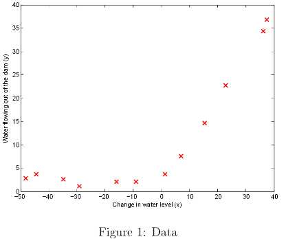
The dataset contains historical records on the change in the water level, x, and the amount of water flowing out of the dam,y.
This dataset is divided into three parts:
(1) plot the training data:
Next:
(1) Implement linear regression and use that to fit a straight line to the data and plot learning curves;
(2) Implement polynomial regression to find a better fit to the data;
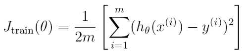
Recall that the regularized linear regression has the following cost function:
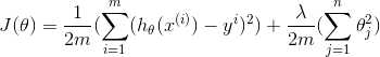
where λ is a regularization parameter which controls the degree of regularization(thus, help preventing overfitting). The regularization term puts a penalty on the overal cost J. As the magnitudes of the model paprameters θj increase, the penalty increase as well. Note that you should not regularize the θ0 term.
Correspondingly, the partial derivative of regularized linear regression‘s cost for θj is defined as:
the file linearRegCostFunction.m:
function [J, grad] = linearRegCostFunction(X, y, theta, lambda)
%LINEARREGCOSTFUNCTION Compute cost and gradient for regularized linear
%regression with multiple variables
%   [J, grad] = LINEARREGCOSTFUNCTION(X, y, theta, lambda) computes the
%   cost of using theta as the parameter for linear regression to fit the
%   data points in X and y. Returns the cost in J and the gradient in grad

% Initialize some useful values
m = length(y); % number of training examples

% You need to return the following variables correctly
J = 0;
grad = zeros(size(theta));

% ====================== YOUR CODE HERE ======================
% Instructions: Compute the cost and gradient of regularized linear
%               regression for a particular choice of theta.
%
%               You should set J to the cost and grad to the gradient.
%

%cost function
hx = X*theta;
J = (1/(2*m))*sumsq(hx-y);
reg = lambda/(2*m)*sumsq(theta(2:end));
J = J + reg;
%gradient
% Part 1.3
grad = (X‘ * (hx-y)) / m;
grad(2:end) +=  lambda * theta(2:end) / m;
% =========================================================================

grad = grad(:);

end
Once your cost function and gradient are working correctly, the next part is to run the code in trainLinearReg.m to compute the optimal values of θ. This training function uses fmincg to optimize the cost function:
function [theta] = trainLinearReg(X, y, lambda)
%TRAINLINEARREG Trains linear regression given a dataset (X, y) and a
%regularization parameter lambda
%   [theta] = TRAINLINEARREG (X, y, lambda) trains linear regression using
%   the dataset (X, y) and regularization parameter lambda. Returns the
%   trained parameters theta.
%

% Initialize Theta
initial_theta = zeros(size(X, 2), 1);

% Create "short hand" for the cost function to be minimized
costFunction = @(t) linearRegCostFunction(X, y, t, lambda);

% Now, costFunction is a function that takes in only one argument
options = optimset(‘MaxIter‘, 200, ‘GradObj‘, ‘on‘);

% Minimize using fmincg
theta = fmincg(costFunction, initial_theta, options);

end
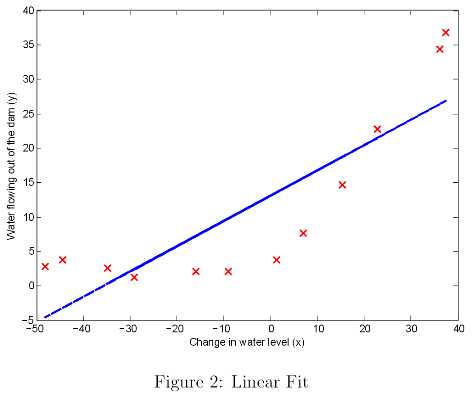
In this part, we set regularization parameter λ to zero. Because our current implementation of linear regression is trying to fit a 2-dimensional θ, regularization will not be incredibly helpful for a θ of such low dimension. In the later parts of the exercise, you will be using polynomial regression with regularization.
Finally we will plot the best fit line, resulting in an image similar to Figure 2.
While visualizing the best fit as shown in one possible way to debug your learing algorithm, it is not always easy to visualize the data and model. In the next section, you will implement a function to generate learing curves that can help you debug your learining algorithm even if it is not easy to visualize the data.
An important concept in machine learning is the bias-vairance tradeoff.Models with high bias are not complex enough for the data and tend to underfit, while models with high variance overfit to the training data.
In this part, we will plot training and test errors on a learning curve to diagnose bias-variance problems.
A learning curve plots training and cross validation error as a function of training set size. learningCurve.m returns a vector of errors for the training set and cross validation set.
To plot the learning curve, we need a training and cross validation set error for different training set sizes. To obtain different training set sizes, we should use different subsets of the original training set X.
We can use the trainLinearReg function to find the θ parameters. Note that the lambda is passed as a parameter to the learningCurve function. After learning the θ parameters, we should compute the error on the training and cross validation sets. Recall that the training error for a dataset is defined as:
In particular, note that the training error does not include the regularization term. One way to compute the training error is to use exsiting cost function and set λ to 0 only when using it to compute the training error and cross validation error. When we are computing the training set error, make sure you compute it on the training subset instead of the entire training set. However, for the cross validation error, we should compute it over the entire validation set.
When we are finished, we will see a plot similar to Figure 3.
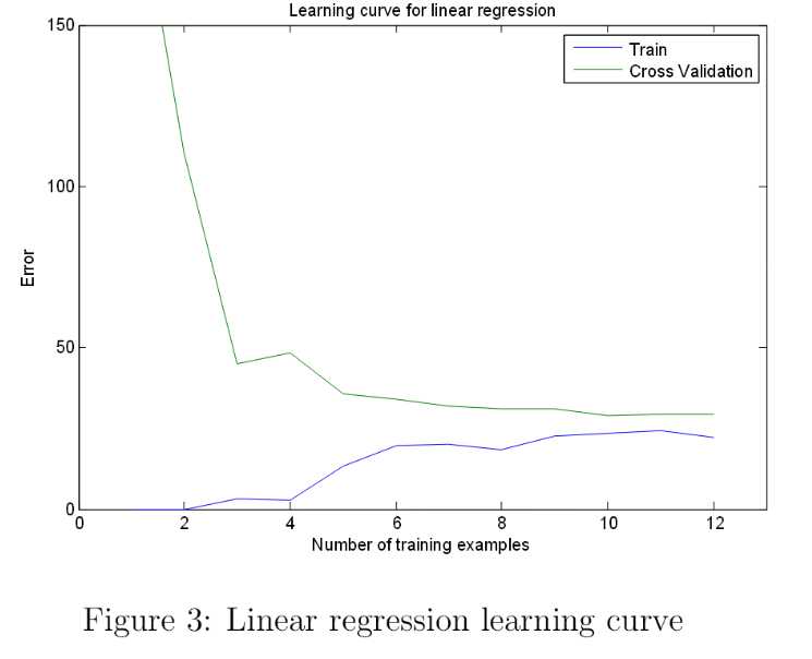
In Figure 3, we can observe that both the training error and cross validation error are high when the number of training examples is increased. This reflects a high bias problem in the model -- the linear regression is too simple and is unable to fit our dataset well. In the next section, you will implement polynomial regression to fit a better model for this dataset.
function [error_train, error_val] = ...
    learningCurve(X, y, Xval, yval, lambda)
%LEARNINGCURVE Generates the train and cross validation set errors needed
%to plot a learning curve
%   [error_train, error_val] = ...
%       LEARNINGCURVE(X, y, Xval, yval, lambda) returns the train and
%       cross validation set errors for a learning curve. In particular,
%       it returns two vectors of the same length - error_train and
%       error_val. Then, error_train(i) contains the training error for
%       i examples (and similarly for error_val(i)).
%
%   In this function, you will compute the train and test errors for
%   dataset sizes from 1 up to m. In practice, when working with larger
%   datasets, you might want to do this in larger intervals.
%

% Number of training examples
m = size(X, 1);

% You need to return these values correctly
error_train = zeros(m, 1);
error_val   = zeros(m, 1);

% ====================== YOUR CODE HERE ======================
% Instructions: Fill in this function to return training errors in
%               error_train and the cross validation errors in error_val.
%               i.e., error_train(i) and
%               error_val(i) should give you the errors
%               obtained after training on i examples.
%
% Note: You should evaluate the training error on the first i training
%       examples (i.e., X(1:i, :) and y(1:i)).
%
%       For the cross-validation error, you should instead evaluate on
%       the _entire_ cross validation set (Xval and yval).
%
% Note: If you are using your cost function (linearRegCostFunction)
%       to compute the training and cross validation error, you should
%       call the function with the lambda argument set to 0.
%       Do note that you will still need to use lambda when running
%       the training to obtain the theta parameters.
%
% Hint: You can loop over the examples with the following:
%
%       for i = 1:m
%           % Compute train/cross validation errors using training examples
%           % X(1:i, :) and y(1:i), storing the result in
%           % error_train(i) and error_val(i)
%           ....
%
%       end
%

% ---------------------- Sample Solution ----------------------
for i = 1:m,
  [theta] = trainLinearReg(X(1:i,:),y(1:i),lambda);
  error_train(i) = linearRegCostFunction(X(1:i,:),y(1:i),theta,0);
  error_val(i) = linearRegCostFunction(Xval,yval,theta,0);
end;
% -------------------------------------------------------------

% =========================================================================

end
The problem with our linear model was that it was too simple for the data and resulted in underfitting(high bias). In this part of the exercise, we will address this problem by adding more features.
Our hypothesis has the form:

We obtain a linear regression model where the features are the various powers of the original value(waterLevel). Complete the code in polyFeatures.m so that the function maps the original training set X of size m*1 into its higher powers. Specifically, when a training set X of size m*1 is passed into the function, the function should reture a m*p matrix X_poly, where column 1 holds the original values of X, column 2 holds the values of X.^2, column 3 holds the values of X.^3, and so on. Now we have a function that will map features to a higher dimension.
function [X_poly] = polyFeatures(X, p)
%POLYFEATURES Maps X (1D vector) into the p-th power
%   [X_poly] = POLYFEATURES(X, p) takes a data matrix X (size m x 1) and
%   maps each example into its polynomial features where
%   X_poly(i, :) = [X(i) X(i).^2 X(i).^3 ...  X(i).^p];
%
% You need to return the following variables correctly.
X_poly = zeros(numel(X), p);

% ====================== YOUR CODE HERE ======================
% Instructions: Given a vector X, return a matrix X_poly where the p-th
%               column of X contains the values of X to the p-th power.
%
%

for i=1:p
  X_poly(:,i) = X.^i;
end;
% =========================================================================

end
Before we are still solving a linear regressino optimization problem.
In this part, we will be using a polynomial of degree 8. It turns out that if we run the training directly on the projected data, will not work well as the features would be badly scaled(e.g., an example with x=40 will now have a feature x8=408=6.5*1012). There fore, we will need to use feature normalization. Call featureNormalize and normalize the features of the training set, storing the mu, sigma parameters separately.
function [X_norm, mu, sigma] = featureNormalize(X)
%FEATURENORMALIZE Normalizes the features in X
%   FEATURENORMALIZE(X) returns a normalized version of X where
%   the mean value of each feature is 0 and the standard deviation
%   is 1. This is often a good preprocessing step to do when
%   working with learning algorithms.

mu = mean(X);
X_norm = bsxfun(@minus, X, mu);

sigma = std(X_norm);
X_norm = bsxfun(@rdivide, X_norm, sigma);

% ============================================================

end
After learning the parameters θ, we we see two plots(Figure 4,5) generated for polynomial regression with λ=0.
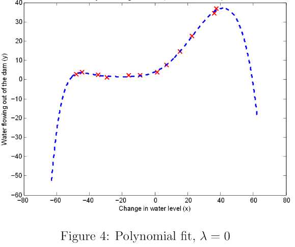
From Figure 4, we should see that the poly nomial fit is able to follow the datapoints very well - thus, obtaining a low training error. However, the polynomial fit is very complex and even drops off at the extremes. This is an indicator that the polynomial regression model is overfitting the training data and will not generalize well.
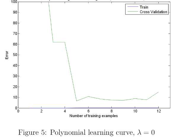
Figure 5 shows the same effect where the low training error is low, but the cross validation error is high. There is a gap between the training and cross validation errors, indicating a high variance problem.
One way to combat the overfitting(hight-variance) problem is to add regularization to the model.
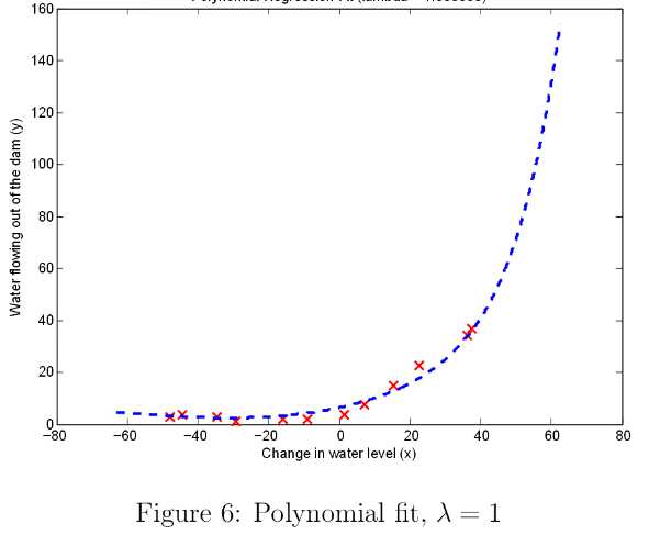
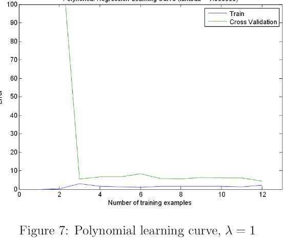
In this section, we will get to observe how the regularization parameter affects the bias-vairance of regularized polynomial regression. Modify the lambda parameter and try λ=1,100.
For λ=1, we should see a polynomial fit that follows the data trend well(Figure 6) and a learning curve(Figure 7) showing that both the cross validation and training error converge to a relatively low value. This shows the λ=1 regularized polynomial regression model does not have the high bias or high variance problems. In effect, it achieves a good trade-off between bias and variance.
For λ=100, we should see a polynomial fit(Figure 8) that does not follow the data well. In this case, there is too much regularization and the model is unable to fit the training data.
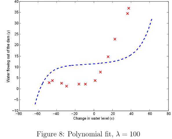
A model without regularization(λ=0) fits the training set well, but does not generalize. Conversely, a model with too much regularization(λ=100) does not fit the training set and testing set well.
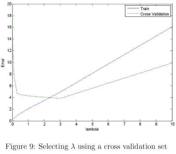
We will use a validation set to evaluate how good each λ value is. After selecting the best λ value using the cross validation set, we an then evaluate the model on teh test set to estimate how well the model will perform on actual unseen data.
We should use the trainLinearReg function to train the model using different values of λ and compute the train error and cross validation error. Try λ in the following range:{0,0.001,0.003,0.01,0.03,0.1,0.3,1,3,10}.
validationCurve.m:
function [lambda_vec, error_train, error_val] = ...
    validationCurve(X, y, Xval, yval)
%VALIDATIONCURVE Generate the train and validation errors needed to
%plot a validation curve that we can use to select lambda
%   [lambda_vec, error_train, error_val] = ...
%       VALIDATIONCURVE(X, y, Xval, yval) returns the train
%       and validation errors (in error_train, error_val)
%       for different values of lambda. You are given the training set (X,
%       y) and validation set (Xval, yval).
%

% Selected values of lambda (you should not change this)
lambda_vec = [0 0.001 0.003 0.01 0.03 0.1 0.3 1 3 10]‘;

% You need to return these variables correctly.
error_train = zeros(length(lambda_vec), 1);
error_val = zeros(length(lambda_vec), 1);

% ====================== YOUR CODE HERE ======================
% Instructions: Fill in this function to return training errors in
%               error_train and the validation errors in error_val. The
%               vector lambda_vec contains the different lambda parameters
%               to use for each calculation of the errors, i.e,
%               error_train(i), and error_val(i) should give
%               you the errors obtained after training with
%               lambda = lambda_vec(i)
%
% Note: You can loop over lambda_vec with the following:
%
%       for i = 1:length(lambda_vec)
%           lambda = lambda_vec(i);
%           % Compute train / val errors when training linear
%           % regression with regularization parameter lambda
%           % You should store the result in error_train(i)
%           % and error_val(i)
%           ....
%
%       end
%
%

for i = 1:length(lambda_vec),
    lambda = lambda_vec(i);
    theta = trainLinearReg(X, y, lambda);
    error_train(i) = linearRegCostFunction(X, y, theta, 0);
    error_val(i) = linearRegCostFunction(Xval, yval, theta, 0);
end;

% =========================================================================

end
We should see a plot similar to Figure 9. In this figure, we can see that the best value of λ is around 3. Due to randomness in the training and validation splits of the dataset, the cross validation error can sometimes be lower thatn the training error.
To get a better indication of the model‘s performance in the real world, it is important to evaluate the "final" model on a test set that was not used in any part of training.
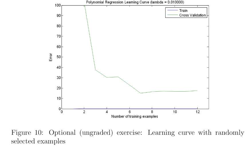
In practivce, especially for small training sets, when you polt learning curves to debug your algorithms, it is often helpful to average across multiple sets of randomly selected examples to determin the training error and cross validation error.
Concretely, to determine the training error and cross validation error for i examples, you should first randomly select i examples from the training set and i examples from the cross validation set. We will then learn the parameters θ on the randomly chosen training set and evaluate the parameters θ using the randomly chosen training set and cross validation set. The above steps should then be repeated multiple times and averaged error should be used to determine the training error and cross validation error for i examples.
Figure 10 shows the learning curve we obtained for polynomial regression with λ=0.01.
标签:
原文地址:http://www.cnblogs.com/CheeseZH/p/4673488.html