使用神经网络来识别手写数字【转译】（二）

时间：2016-03-26 13:53:55 阅读：734 评论：0 收藏：0 [点我收藏+]

标签：

A simple network to classify handwritten digits

Having defined neural networks, let‘s return to handwriting recognition. We can split the problem of recognizing handwritten digits into two sub-problems. First, we‘d like a way of breaking an image containing many digits into a sequence of separate images, each containing a single digit. For example, we‘d like to break the image

into six separate images,

We humans solve this segmentation problem with ease, but it‘s challenging for a computer program to correctly break up the image. Once the image has been segmented, the program then needs to classify each individual digit. So, for instance, we‘d like our program to recognize that the first digit above,

is a 5.

We‘ll focus on writing a program to solve the second problem, that is, classifying individual digits. We do this because it turns out that the segmentation problem is not so difficult to solve, once you have a good way of classifying individual digits. There are many approaches to solving the segmentation problem. One approach is to trial many different ways of segmenting the image, using the individual digit classifier to score each trial segmentation. A trial segmentation gets a high score if the individual digit classifier is confident of its classification in all segments, and a low score if the classifier is having a lot of trouble in one or more segments. The idea is that if the classifier is having trouble somewhere, then it‘s probably having trouble because the segmentation has been chosen incorrectly. This idea and other variations can be used to solve the segmentation problem quite well. So instead of worrying about segmentation we‘ll concentrate on developing a neural network which can solve the more interesting and difficult problem, namely, recognizing individual handwritten digits.

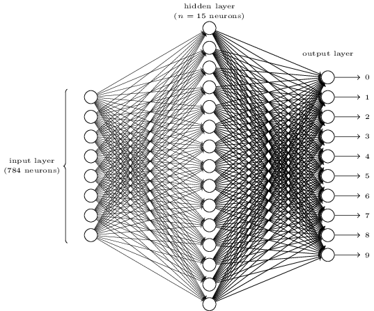
To recognize individual digits we will use a three-layer neural network:

The input layer of the network contains neurons encoding the values of the input pixels. As discussed in the next section, our training data for the network will consist of many

The second layer of the network is a hidden layer. We denote the number of neurons in this hidden layer by

The output layer of the network contains 10 neurons. If the first neuron fires, i.e., has an output

You might wonder why we use

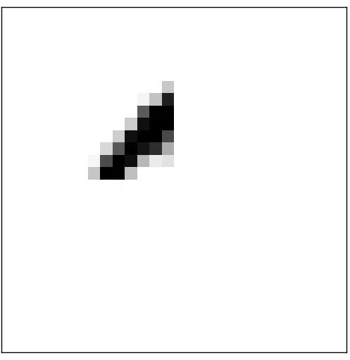
To understand why we do this, it helps to think about what the neural network is doing from first principles. Consider first the case where we use

It can do this by heavily weighting input pixels which overlap with the image, and only lightly weighting the other inputs. In a similar way, let‘s suppose for the sake of argument that the second, third, and fourth neurons in the hidden layer detect whether or not the following images are present:

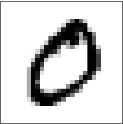
As you may have guessed, these four images together make up the

So if all four of these hidden neurons are firing then we can conclude that the digit is a

Supposing the neural network functions in this way, we can give a plausible explanation for why it‘s better to have

Now, with all that said, this is all just a heuristic. Nothing says that the three-layer neural network has to operate in the way I described, with the hidden neurons detecting simple component shapes. Maybe a clever learning algorithm will find some assignment of weights that lets us use only

Exercise

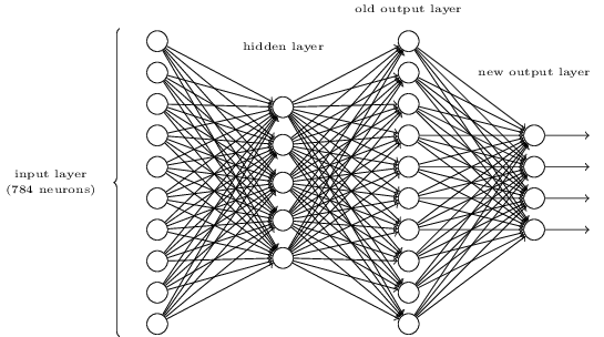
There is a way of determining the bitwise representation of a digit by adding an extra layer to the three-layer network above. The extra layer converts the output from the previous layer into a binary representation, as illustrated in the figure below. Find a set of weights and biases for the new output layer. Assume that the first

Learning with gradient descent

Now that we have a design for our neural network, how can it learn to recognize digits? The first thing we‘ll need is a data set to learn from - a so-called training data set. We‘ll use the MNIST data set, which contains tens of thousands of scanned images of handwritten digits, together with their correct classifications. MNIST‘s name comes from the fact that it is a modified subset of two data sets collected by NIST, the United States‘ National Institute of Standards and Technology. Here‘s a few images from MNIST:

As you can see, these digits are, in fact, the same as those shown at the beginning of this chapter as a challenge to recognize. Of course, when testing our network we‘ll ask it to recognize images which aren‘t in the training set!

The MNIST data comes in two parts. The first part contains 60,000 images to be used as training data. These images are scanned handwriting samples from 250 people, half of whom were US Census Bureau employees, and half of whom were high school students. The images are greyscale and 28 by 28 pixels in size. The second part of the MNIST data set is 10,000 images to be used as test data. Again, these are 28 by 28 greyscale images. We‘ll use the test data to evaluate how well our neural network has learned to recognize digits. To make this a good test of performance, the test data was taken from a different set of 250 people than the original training data (albeit still a group split between Census Bureau employees and high school students). This helps give us confidence that our system can recognize digits from people whose writing it didn‘t see during training.

We‘ll use the notation

What we‘d like is an algorithm which lets us find weights and biases so that the output from the network approximates

C (w, b) \equiv 1 2 n \sum x ∥ y ( x ) - a ∥ 2 . (6)

Why introduce the quadratic cost? After all, aren‘t we primarily interested in the number of images correctly classified by the network? Why not try to maximize that number directly, rather than minimizing a proxy measure like the quadratic cost? The problem with that is that the number of images correctly classified is not a smooth function of the weights and biases in the network. For the most part, making small changes to the weights and biases won‘t cause any change at all in the number of training images classified correctly. That makes it difficult to figure out how to change the weights and biases to get improved performance. If we instead use a smooth cost function like the quadratic cost it turns out to be easy to figure out how to make small changes in the weights and biases so as to get an improvement in the cost. That‘s why we focus first on minimizing the quadratic cost, and only after that will we examine the classification accuracy.

Even given that we want to use a smooth cost function, you may still wonder why we choose the quadratic function used in Equation (6). Isn‘t this a rather ad hoc choice? Perhaps if we chose a different cost function we‘d get a totally different set of minimizing weights and biases? This is a valid concern, and later we‘ll revisit the cost function, and make some modifications. However, the quadratic cost function of Equation (6) works perfectly well for understanding the basics of learning in neural networks, so we‘ll stick with it for now.

Recapping, our goal in training a neural network is to find weights and biases which minimize the quadratic cost function

Okay, let‘s suppose we‘re trying to minimize some function,

What we‘d like is to find where

One way of attacking the problem is to use calculus to try to find the minimum analytically. We could compute derivatives and then try using them to find places where

(After asserting that we‘ll gain insight by imagining

Okay, so calculus doesn‘t work. Fortunately, there is a beautiful analogy which suggests an algorithm which works pretty well. We start by thinking of our function as a kind of a valley. If you squint just a little at the plot above, that shouldn‘t be too hard. And we imagine a ball rolling down the slope of the valley. Our everyday experience tells us that the ball will eventually roll to the bottom of the valley. Perhaps we can use this idea as a way to find a minimum for the function? We‘d randomly choose a starting point for an (imaginary) ball, and then simulate the motion of the ball as it rolled down to the bottom of the valley. We could do this simulation simply by computing derivatives (and perhaps some second derivatives) of

Based on what I‘ve just written, you might suppose that we‘ll be trying to write down Newton‘s equations of motion for the ball, considering the effects of friction and gravity, and so on. Actually, we‘re not going to take the ball-rolling analogy quite that seriously - we‘re devising an algorithm to minimize

To make this question more precise, let‘s think about what happens when we move the ball a small amount

Δ C \approx \partial C \partial v 1 Δ v 1 + \partial C \partial v 2 Δ v 2 . (7)

\nabla C \equiv (\partial C \partial v 1 , \partial C \partial v 2 ) T . (8)

With these definitions, the expression (7) for

Δ C \approx \nabla C \cdot Δ v . (9)

Δ v = - η \nabla C, (10)

v \to v' = v - η \nabla C . (11)

Summing up, the way the gradient descent algorithm works is to repeatedly compute the gradient

Notice that with this rule gradient descent doesn‘t reproduce real physical motion. In real life a ball has momentum, and that momentum may allow it to roll across the slope, or even (momentarily) roll uphill. It‘s only after the effects of friction set in that the ball is guaranteed to roll down into the valley. By contrast, our rule for choosing

To make gradient descent work correctly, we need to choose the learning rate

I‘ve explained gradient descent when

Δ C \approx \nabla C \cdot Δ v, (12)

\nabla C \equiv (\partial C \partial v 1 , \dots , \partial C \partial v m ) T . (13)

Δ v = - η \nabla C, (14)

v \to v' = v - η \nabla C . (15)

Indeed, there‘s even a sense in which gradient descent is the optimal strategy for searching for a minimum. Let‘s suppose that we‘re trying to make a move

Exercises

Prove the assertion of the last paragraph. Hint: If you‘re not already familiar with the Cauchy-Schwarz inequality, you may find it helpful to familiarize yourself with it.
I explained gradient descent when

People have investigated many variations of gradient descent, including variations that more closely mimic a real physical ball. These ball-mimicking variations have some advantages, but also have a major disadvantage: it turns out to be necessary to compute second partial derivatives of

How can we apply gradient descent to learn in a neural network? The idea is to use gradient descent to find the weights

w k b l \to \to w' k = w k - η \partial C \partial w k b ' l

There are a number of challenges in applying the gradient descent rule. We‘ll look into those in depth in later chapters. But for now I just want to mention one problem. To understand what the problem is, let‘s look back at the quadratic cost in Equation (6). Notice that this cost function has the form

An idea called stochastic gradient descent can be used to speed up learning. The idea is to estimate the gradient

To make these ideas more precise, stochastic gradient descent works by randomly picking out a small number

\sum m j = 1 \nabla C X j m \approx \sum x \nabla C x n = \nabla C , (18)

\nabla C \approx 1 m \sum j = 1 m \nabla C X j , (19)

To connect this explicitly to learning in neural networks, suppose

w k b l \to \to w' k = w k - η m \sum j \partial C X

Incidentally, it‘s worth noting that conventions vary about scaling of the cost function and of mini-batch updates to the weights and biases. In Equation (6) we scaled the overall cost function by a factor

We can think of stochastic gradient descent as being like political polling: it‘s much easier to sample a small mini-batch than it is to apply gradient descent to the full batch, just as carrying out a poll is easier than running a full election. For example, if we have a training set of size

Exercise

An extreme version of gradient descent is to use a mini-batch size of just 1. That is, given a training input,

Let me conclude this section by discussing a point that sometimes bugs people new to gradient descent. In neural networks the cost

Implementing our network to classify digits

Alright, let‘s write a program that learns how to recognize handwritten digits, using stochastic gradient descent and the MNIST training data. We‘ll do this with a short Python (2.7) program, just 74 lines of code! The first thing we need is to get the MNIST data. If you‘re a git user then you can obtain the data by cloning the code repository for this book,

git clone https://github.com/mnielsen/neural-networks-and-deep-learning.git

If you don‘t use git then you can download the data and code here.

Incidentally, when I described the MNIST data earlier, I said it was split into 60,000 training images, and 10,000 test images. That‘s the official MNIST description. Actually, we‘re going to split the data a little differently. We‘ll leave the test images as is, but split the 60,000-image MNIST training set into two parts: a set of 50,000 images, which we‘ll use to train our neural network, and a separate 10,000 image validation set. We won‘t use the validation data in this chapter, but later in the book we‘ll find it useful in figuring out how to set certain hyper-parameters of the neural network - things like the learning rate, and so on, which aren‘t directly selected by our learning algorithm. Although the validation data isn‘t part of the original MNIST specification, many people use MNIST in this fashion, and the use of validation data is common in neural networks. When I refer to the "MNIST training data" from now on, I‘ll be referring to our 50,000 image data set, not the original 60,000 image data set**As noted earlier, the MNIST data set is based on two data sets collected by NIST, the United States‘ National Institute of Standards and Technology. To construct MNIST the NIST data sets were stripped down and put into a more convenient format by Yann LeCun, Corinna Cortes, and Christopher J. C. Burges. See this link for more details. The data set in my repository is in a form that makes it easy to load and manipulate the MNIST data in Python. I obtained this particular form of the data from the LISA machine learning laboratory at the University of Montreal (link)..

Apart from the MNIST data we also need a Python library calledNumpy, for doing fast linear algebra. If you don‘t already have Numpy installed, you can get it here.

Let me explain the core features of the neural networks code, before giving a full listing, below. The centerpiece is a Network class, which we use to represent a neural network. Here‘s the code we use to initialize a Network object:

class Network(object):

    def __init__(self, sizes):
        self.num_layers = len(sizes)
        self.sizes = sizes
        self.biases = [np.random.randn(y, 1) for y in sizes[1:]]
        self.weights = [np.random.randn(y, x) 
                        for x, y in zip(sizes[:-1], sizes[1:])]

In this code, the list sizes contains the number of neurons in the respective layers. So, for example, if we want to create a Networkobject with 2 neurons in the first layer, 3 neurons in the second layer, and 1 neuron in the final layer, we‘d do this with the code:

net = Network([2, 3, 1])

Note also that the biases and weights are stored as lists of Numpy matrices. So, for example net.weights[1] is a Numpy matrix storing the weights connecting the second and third layers of neurons. (It‘s not the first and second layers, since Python‘s list indexing starts at0.) Since net.weights[1] is rather verbose, let‘s just denote that matrix

a' = σ (w a + b) . (22)

Exercise

Write out Equation (22) in component form, and verify that it gives the same result as the rule (4) for computing the output of a sigmoid neuron.

With all this in mind, it‘s easy to write code computing the output from a Network instance. We begin by defining the sigmoid function:

def sigmoid(z):
    return 1.0/(1.0+np.exp(-z))

We then add a feedforward method to the Network class, which, given an input a for the network, returns the corresponding output**It is assumed that the input a is an (n, 1)Numpy ndarray, not a (n,) vector. Here, n is the number of inputs to the network. If you try to use an (n,) vector as input you‘ll get strange results. Although using an (n,) vector appears the more natural choice, using an (n, 1) ndarray makes it particularly easy to modify the code to feedforward multiple inputs at once, and that is sometimes convenient.. All the method does is applies Equation (22) for each layer:

    def feedforward(self, a):
        """Return the output of the network if "a" is input."""
        for b, w in zip(self.biases, self.weights):
            a = sigmoid(np.dot(w, a)+b)
        return a

Of course, the main thing we want our Network objects to do is to learn. To that end we‘ll give them an SGD method which implements stochastic gradient descent. Here‘s the code. It‘s a little mysterious in a few places, but I‘ll break it down below, after the listing.

    def SGD(self, training_data, epochs, mini_batch_size, eta,
            test_data=None):
        """Train the neural network using mini-batch stochastic
        gradient descent.  The "training_data" is a list of tuples
        "(x, y)" representing the training inputs and the desired
        outputs.  The other non-optional parameters are
        self-explanatory.  If "test_data" is provided then the
        network will be evaluated against the test data after each
        epoch, and partial progress printed out.  This is useful for
        tracking progress, but slows things down substantially."""
        if test_data: n_test = len(test_data)
        n = len(training_data)
        for j in xrange(epochs):
            random.shuffle(training_data)
            mini_batches = [
                training_data[k:k+mini_batch_size]
                for k in xrange(0, n, mini_batch_size)]
            for mini_batch in mini_batches:
                self.update_mini_batch(mini_batch, eta)
            if test_data:
                print "Epoch {0}: {1} / {2}".format(
                    j, self.evaluate(test_data), n_test)
            else:
                print "Epoch {0} complete".format(j)

The training_data is a list of tuples (x, y) representing the training inputs and corresponding desired outputs. The variables epochs andmini_batch_size are what you‘d expect - the number of epochs to train for, and the size of the mini-batches to use when sampling. eta is the learning rate,

The code works as follows. In each epoch, it starts by randomly shuffling the training data, and then partitions it into mini-batches of the appropriate size. This is an easy way of sampling randomly from the training data. Then for each mini_batch we apply a single step of gradient descent. This is done by the codeself.update_mini_batch(mini_batch, eta), which updates the network weights and biases according to a single iteration of gradient descent, using just the training data in mini_batch. Here‘s the code for the update_mini_batch method:

    def update_mini_batch(self, mini_batch, eta):
        """Update the network‘s weights and biases by applying
        gradient descent using backpropagation to a single mini batch.
        The "mini_batch" is a list of tuples "(x, y)", and "eta"
        is the learning rate."""
        nabla_b = [np.zeros(b.shape) for b in self.biases]
        nabla_w = [np.zeros(w.shape) for w in self.weights]
        for x, y in mini_batch:
            delta_nabla_b, delta_nabla_w = self.backprop(x, y)
            nabla_b = [nb+dnb for nb, dnb in zip(nabla_b, delta_nabla_b)]
            nabla_w = [nw+dnw for nw, dnw in zip(nabla_w, delta_nabla_w)]
        self.weights = [w-(eta/len(mini_batch))*nw 
                        for w, nw in zip(self.weights, nabla_w)]
        self.biases = [b-(eta/len(mini_batch))*nb 
                       for b, nb in zip(self.biases, nabla_b)]

            delta_nabla_b, delta_nabla_w = self.backprop(x, y)

I‘m not going to show the code for self.backprop right now. We‘ll study how backpropagation works in the next chapter, including the code for self.backprop. For now, just assume that it behaves as claimed, returning the appropriate gradient for the cost associated to the training example x.

Let‘s look at the full program, including the documentation strings, which I omitted above. Apart from self.backprop the program is self-explanatory - all the heavy lifting is done in self.SGD andself.update_mini_batch, which we‘ve already discussed. Theself.backprop method makes use of a few extra functions to help in computing the gradient, namely sigmoid_prime, which computes the derivative of the

"""
network.py
~~~~~~~~~~

A module to implement the stochastic gradient descent learning
algorithm for a feedforward neural network.  Gradients are calculated
using backpropagation.  Note that I have focused on making the code
simple, easily readable, and easily modifiable.  It is not optimized,
and omits many desirable features.
"""

#### Libraries
# Standard library
import random

# Third-party libraries
import numpy as np

class Network(object):

    def __init__(self, sizes):
        """The list ``sizes`` contains the number of neurons in the
        respective layers of the network.  For example, if the list
        was [2, 3, 1] then it would be a three-layer network, with the
        first layer containing 2 neurons, the second layer 3 neurons,
        and the third layer 1 neuron.  The biases and weights for the
        network are initialized randomly, using a Gaussian
        distribution with mean 0, and variance 1.  Note that the first
        layer is assumed to be an input layer, and by convention we
        won‘t set any biases for those neurons, since biases are only
        ever used in computing the outputs from later layers."""
        self.num_layers = len(sizes)
        self.sizes = sizes
        self.biases = [np.random.randn(y, 1) for y in sizes[1:]]
        self.weights = [np.random.randn(y, x)
                        for x, y in zip(sizes[:-1], sizes[1:])]

    def feedforward(self, a):
        """Return the output of the network if ``a`` is input."""
        for b, w in zip(self.biases, self.weights):
            a = sigmoid(np.dot(w, a)+b)
        return a

    def SGD(self, training_data, epochs, mini_batch_size, eta,
            test_data=None):
        """Train the neural network using mini-batch stochastic
        gradient descent.  The ``training_data`` is a list of tuples
        ``(x, y)`` representing the training inputs and the desired
        outputs.  The other non-optional parameters are
        self-explanatory.  If ``test_data`` is provided then the
        network will be evaluated against the test data after each
        epoch, and partial progress printed out.  This is useful for
        tracking progress, but slows things down substantially."""
        if test_data: n_test = len(test_data)
        n = len(training_data)
        for j in xrange(epochs):
            random.shuffle(training_data)
            mini_batches = [
                training_data[k:k+mini_batch_size]
                for k in xrange(0, n, mini_batch_size)]
            for mini_batch in mini_batches:
                self.update_mini_batch(mini_batch, eta)
            if test_data:
                print "Epoch {0}: {1} / {2}".format(
                    j, self.evaluate(test_data), n_test)
            else:
                print "Epoch {0} complete".format(j)

    def update_mini_batch(self, mini_batch, eta):
        """Update the network‘s weights and biases by applying
        gradient descent using backpropagation to a single mini batch.
        The ``mini_batch`` is a list of tuples ``(x, y)``, and ``eta``
        is the learning rate."""
        nabla_b = [np.zeros(b.shape) for b in self.biases]
        nabla_w = [np.zeros(w.shape) for w in self.weights]
        for x, y in mini_batch:
            delta_nabla_b, delta_nabla_w = self.backprop(x, y)
            nabla_b = [nb+dnb for nb, dnb in zip(nabla_b, delta_nabla_b)]
            nabla_w = [nw+dnw for nw, dnw in zip(nabla_w, delta_nabla_w)]
        self.weights = [w-(eta/len(mini_batch))*nw
                        for w, nw in zip(self.weights, nabla_w)]
        self.biases = [b-(eta/len(mini_batch))*nb
                       for b, nb in zip(self.biases, nabla_b)]

    def backprop(self, x, y):
        """Return a tuple ``(nabla_b, nabla_w)`` representing the
        gradient for the cost function C_x.  ``nabla_b`` and
        ``nabla_w`` are layer-by-layer lists of numpy arrays, similar
        to ``self.biases`` and ``self.weights``."""
        nabla_b = [np.zeros(b.shape) for b in self.biases]
        nabla_w = [np.zeros(w.shape) for w in self.weights]
        # feedforward
        activation = x
        activations = [x] # list to store all the activations, layer by layer
        zs = [] # list to store all the z vectors, layer by layer
        for b, w in zip(self.biases, self.weights):
            z = np.dot(w, activation)+b
            zs.append(z)
            activation = sigmoid(z)
            activations.append(activation)
        # backward pass
        delta = self.cost_derivative(activations[-1], y) *             sigmoid_prime(zs[-1])
        nabla_b[-1] = delta
        nabla_w[-1] = np.dot(delta, activations[-2].transpose())
        # Note that the variable l in the loop below is used a little
        # differently to the notation in Chapter 2 of the book.  Here,
        # l = 1 means the last layer of neurons, l = 2 is the
        # second-last layer, and so on.  It‘s a renumbering of the
        # scheme in the book, used here to take advantage of the fact
        # that Python can use negative indices in lists.
        for l in xrange(2, self.num_layers):
            z = zs[-l]
            sp = sigmoid_prime(z)
            delta = np.dot(self.weights[-l+1].transpose(), delta) * sp
            nabla_b[-l] = delta
            nabla_w[-l] = np.dot(delta, activations[-l-1].transpose())
        return (nabla_b, nabla_w)

    def evaluate(self, test_data):
        """Return the number of test inputs for which the neural
        network outputs the correct result. Note that the neural
        network‘s output is assumed to be the index of whichever
        neuron in the final layer has the highest activation."""
        test_results = [(np.argmax(self.feedforward(x)), y)
                        for (x, y) in test_data]
        return sum(int(x == y) for (x, y) in test_results)

    def cost_derivative(self, output_activations, y):
        """Return the vector of partial derivatives \partial C_x /
        \partial a for the output activations."""
        return (output_activations-y)

#### Miscellaneous functions
def sigmoid(z):
    """The sigmoid function."""
    return 1.0/(1.0+np.exp(-z))

def sigmoid_prime(z):
    """Derivative of the sigmoid function."""
    return sigmoid(z)*(1-sigmoid(z))

How well does the program recognize handwritten digits? Well, let‘s start by loading in the MNIST data. I‘ll do this using a little helper program, mnist_loader.py, to be described below. We execute the following commands in a Python shell,

>>> import mnist_loader
>>> training_data, validation_data, test_data = ... mnist_loader.load_data_wrapper()

Of course, this could also be done in a separate Python program, but if you‘re following along it‘s probably easiest to do in a Python shell.

After loading the MNIST data, we‘ll set up a Network with

>>> import network
>>> net = network.Network([784, 30, 10])

Finally, we‘ll use stochastic gradient descent to learn from the MNIST training_data over 30 epochs, with a mini-batch size of 10, and a learning rate of

>>> net.SGD(training_data, 30, 10, 3.0, test_data=test_data)

Note that if you‘re running the code as you read along, it will take some time to execute - for a typical machine (as of 2015) it will likely take a few minutes to run. I suggest you set things running, continue to read, and periodically check the output from the code. If you‘re in a rush you can speed things up by decreasing the number of epochs, by decreasing the number of hidden neurons, or by using only part of the training data. Note that production code would be much, much faster: these Python scripts are intended to help you understand how neural nets work, not to be high-performance code! And, of course, once we‘ve trained a network it can be run very quickly indeed, on almost any computing platform. For example, once we‘ve learned a good set of weights and biases for a network, it can easily be ported to run in Javascript in a web browser, or as a native app on a mobile device. In any case, here is a partial transcript of the output of one training run of the neural network. The transcript shows the number of test images correctly recognized by the neural network after each epoch of training. As you can see, after just a single epoch this has reached 9,129 out of 10,000, and the number continues to grow,

Epoch 0: 9129 / 10000
Epoch 1: 9295 / 10000
Epoch 2: 9348 / 10000
...
Epoch 27: 9528 / 10000
Epoch 28: 9542 / 10000
Epoch 29: 9534 / 10000

That is, the trained network gives us a classification rate of about

Let‘s rerun the above experiment, changing the number of hidden neurons to

>>> net = network.Network([784, 100, 10])
>>> net.SGD(training_data, 30, 10, 3.0, test_data=test_data)

Sure enough, this improves the results to

Of course, to obtain these accuracies I had to make specific choices for the number of epochs of training, the mini-batch size, and the learning rate,

>>> net = network.Network([784, 100, 10])
>>> net.SGD(training_data, 30, 10, 0.001, test_data=test_data)

The results are much less encouraging,

Epoch 0: 1139 / 10000
Epoch 1: 1136 / 10000
Epoch 2: 1135 / 10000
...
Epoch 27: 2101 / 10000
Epoch 28: 2123 / 10000
Epoch 29: 2142 / 10000

In general, debugging a neural network can be challenging. This is especially true when the initial choice of hyper-parameters produces results no better than random noise. Suppose we try the successful 30 hidden neuron network architecture from earlier, but with the learning rate changed to

>>> net = network.Network([784, 30, 10])
>>> net.SGD(training_data, 30, 10, 100.0, test_data=test_data)

Epoch 0: 1009 / 10000
Epoch 1: 1009 / 10000
Epoch 2: 1009 / 10000
Epoch 3: 1009 / 10000
...
Epoch 27: 982 / 10000
Epoch 28: 982 / 10000
Epoch 29: 982 / 10000

The lesson to take away from this is that debugging a neural network is not trivial, and, just as for ordinary programming, there is an art to it. You need to learn that art of debugging in order to get good results from neural networks. More generally, we need to develop heuristics for choosing good hyper-parameters and a good architecture. We‘ll discuss all these at length through the book, including how I chose the hyper-parameters above.

Exercise

Try creating a network with just two layers - an input and an output layer, no hidden layer - with 784 and 10 neurons, respectively. Train the network using stochastic gradient descent. What classification accuracy can you achieve?

Earlier, I skipped over the details of how the MNIST data is loaded. It‘s pretty straightforward. For completeness, here‘s the code. The data structures used to store the MNIST data are described in the documentation strings - it‘s straightforward stuff, tuples and lists of Numpy ndarray objects (think of them as vectors if you‘re not familiar with ndarrays):

"""
mnist_loader
~~~~~~~~~~~~

A library to load the MNIST image data.  For details of the data
structures that are returned, see the doc strings for ``load_data``
and ``load_data_wrapper``.  In practice, ``load_data_wrapper`` is the
function usually called by our neural network code.
"""

#### Libraries
# Standard library
import cPickle
import gzip

# Third-party libraries
import numpy as np

def load_data():
    """Return the MNIST data as a tuple containing the training data,
    the validation data, and the test data.

    The ``training_data`` is returned as a tuple with two entries.
    The first entry contains the actual training images.  This is a
    numpy ndarray with 50,000 entries.  Each entry is, in turn, a
    numpy ndarray with 784 values, representing the 28 * 28 = 784
    pixels in a single MNIST image.

    The second entry in the ``training_data`` tuple is a numpy ndarray
    containing 50,000 entries.  Those entries are just the digit
    values (0...9) for the corresponding images contained in the first
    entry of the tuple.

    The ``validation_data`` and ``test_data`` are similar, except
    each contains only 10,000 images.

    This is a nice data format, but for use in neural networks it‘s
    helpful to modify the format of the ``training_data`` a little.
    That‘s done in the wrapper function ``load_data_wrapper()``, see
    below.
    """
    f = gzip.open(‘../data/mnist.pkl.gz‘, ‘rb‘)
    training_data, validation_data, test_data = cPickle.load(f)
    f.close()
    return (training_data, validation_data, test_data)

def load_data_wrapper():
    """Return a tuple containing ``(training_data, validation_data,
    test_data)``. Based on ``load_data``, but the format is more
    convenient for use in our implementation of neural networks.

    In particular, ``training_data`` is a list containing 50,000
    2-tuples ``(x, y)``.  ``x`` is a 784-dimensional numpy.ndarray
    containing the input image.  ``y`` is a 10-dimensional
    numpy.ndarray representing the unit vector corresponding to the
    correct digit for ``x``.

    ``validation_data`` and ``test_data`` are lists containing 10,000
    2-tuples ``(x, y)``.  In each case, ``x`` is a 784-dimensional
    numpy.ndarry containing the input image, and ``y`` is the
    corresponding classification, i.e., the digit values (integers)
    corresponding to ``x``.

    Obviously, this means we‘re using slightly different formats for
    the training data and the validation / test data.  These formats
    turn out to be the most convenient for use in our neural network
    code."""
    tr_d, va_d, te_d = load_data()
    training_inputs = [np.reshape(x, (784, 1)) for x in tr_d[0]]
    training_results = [vectorized_result(y) for y in tr_d[1]]
    training_data = zip(training_inputs, training_results)
    validation_inputs = [np.reshape(x, (784, 1)) for x in va_d[0]]
    validation_data = zip(validation_inputs, va_d[1])
    test_inputs = [np.reshape(x, (784, 1)) for x in te_d[0]]
    test_data = zip(test_inputs, te_d[1])
    return (training_data, validation_data, test_data)

def vectorized_result(j):
    """Return a 10-dimensional unit vector with a 1.0 in the jth
    position and zeroes elsewhere.  This is used to convert a digit
    (0...9) into a corresponding desired output from the neural
    network."""
    e = np.zeros((10, 1))
    e[j] = 1.0
    return e

I said above that our program gets pretty good results. What does that mean? Good compared to what? It‘s informative to have some simple (non-neural-network) baseline tests to compare against, to understand what it means to perform well. The simplest baseline of all, of course, is to randomly guess the digit. That‘ll be right about ten percent of the time. We‘re doing much better than that!

What about a less trivial baseline? Let‘s try an extremely simple idea: we‘ll look at how dark an image is. For instance, an image of a

This suggests using the training data to compute average darknesses for each digit,

It‘s not difficult to find other ideas which achieve accuracies in the

If we run scikit-learn‘s SVM classifier using the default settings, then it gets 9,435 of 10,000 test images correct. (The code is available here.) That‘s a big improvement over our naive approach of classifying an image based on how dark it is. Indeed, it means that the SVM is performing roughly as well as our neural networks, just a little worse. In later chapters we‘ll introduce new techniques that enable us to improve our neural networks so that they perform much better than the SVM.

That‘s not the end of the story, however. The 9,435 of 10,000 result is for scikit-learn‘s default settings for SVMs. SVMs have a number of tunable parameters, and it‘s possible to search for parameters which improve this out-of-the-box performance. I won‘t explicitly do this search, but instead refer you to this blog post by Andreas Mueller if you‘d like to know more. Mueller shows that with some work optimizing the SVM‘s parameters it‘s possible to get the performance up above 98.5 percent accuracy. In other words, a well-tuned SVM only makes an error on about one digit in 70. That‘s pretty good! Can neural networks do better?

In fact, they can. At present, well-designed neural networks outperform every other technique for solving MNIST, including SVMs. The current (2013) record is classifying 9,979 of 10,000 images correctly. This was done by Li Wan, Matthew Zeiler, Sixin Zhang, Yann LeCun, and Rob Fergus. We‘ll see most of the techniques they used later in the book. At that level the performance is close to human-equivalent, and is arguably better, since quite a few of the MNIST images are difficult even for humans to recognize with confidence, for example:

I trust you‘ll agree that those are tough to classify! With images like these in the MNIST data set it‘s remarkable that neural networks can accurately classify all but 21 of the 10,000 test images. Usually, when programming we believe that solving a complicated problem like recognizing the MNIST digits requires a sophisticated algorithm. But even the neural networks in the Wan et al paper just mentioned involve quite simple algorithms, variations on the algorithm we‘ve seen in this chapter. All the complexity is learned, automatically, from the training data. In some sense, the moral of both our results and those in more sophisticated papers, is that for some problems:

sophisticated algorithm

Toward deep learning

While our neural network gives impressive performance, that performance is somewhat mysterious. The weights and biases in the network were discovered automatically. And that means we don‘t immediately have an explanation of how the network does what it does. Can we find some way to understand the principles by which our network is classifying handwritten digits? And, given such principles, can we do better?

To put these questions more starkly, suppose that a few decades hence neural networks lead to artificial intelligence (AI). Will we understand how such intelligent networks work? Perhaps the networks will be opaque to us, with weights and biases we don‘t understand, because they‘ve been learned automatically. In the early days of AI research people hoped that the effort to build an AI would also help us understand the principles behind intelligence and, maybe, the functioning of the human brain. But perhaps the outcome will be that we end up understanding neither the brain nor how artificial intelligence works!

To address these questions, let‘s think back to the interpretation of artificial neurons that I gave at the start of the chapter, as a means of weighing evidence. Suppose we want to determine whether an image shows a human face or not:

Credits: 1. Ester Inbar. 2. Unknown. 3. NASA, ESA, G. Illingworth, D. Magee, and P. Oesch (University of California, Santa Cruz), R. Bouwens (Leiden University), and the HUDF09 Team. Click on the images for more details.

We could attack this problem the same way we attacked handwriting recognition - by using the pixels in the image as input to a neural network, with the output from the network a single neuron indicating either "Yes, it‘s a face" or "No, it‘s not a face".

Let‘s suppose we do this, but that we‘re not using a learning algorithm. Instead, we‘re going to try to design a network by hand, choosing appropriate weights and biases. How might we go about it? Forgetting neural networks entirely for the moment, a heuristic we could use is to decompose the problem into sub-problems: does the image have an eye in the top left? Does it have an eye in the top right? Does it have a nose in the middle? Does it have a mouth in the bottom middle? Is there hair on top? And so on.

If the answers to several of these questions are "yes", or even just "probably yes", then we‘d conclude that the image is likely to be a face. Conversely, if the answers to most of the questions are "no", then the image probably isn‘t a face.

Of course, this is just a rough heuristic, and it suffers from many deficiencies. Maybe the person is bald, so they have no hair. Maybe we can only see part of the face, or the face is at an angle, so some of the facial features are obscured. Still, the heuristic suggests that if we can solve the sub-problems using neural networks, then perhaps we can build a neural network for face-detection, by combining the networks for the sub-problems. Here‘s a possible architecture, with rectangles denoting the sub-networks. Note that this isn‘t intended as a realistic approach to solving the face-detection problem; rather, it‘s to help us build intuition about how networks function. Here‘s the architecture:

It‘s also plausible that the sub-networks can be decomposed. Suppose we‘re considering the question: "Is there an eye in the top left?" This can be decomposed into questions such as: "Is there an eyebrow?"; "Are there eyelashes?"; "Is there an iris?"; and so on. Of course, these questions should really include positional information, as well - "Is the eyebrow in the top left, and above the iris?", that kind of thing - but let‘s keep it simple. The network to answer the question "Is there an eye in the top left?" can now be decomposed:

Those questions too can be broken down, further and further through multiple layers. Ultimately, we‘ll be working with sub-networks that answer questions so simple they can easily be answered at the level of single pixels. Those questions might, for example, be about the presence or absence of very simple shapes at particular points in the image. Such questions can be answered by single neurons connected to the raw pixels in the image.

The end result is a network which breaks down a very complicated question - does this image show a face or not - into very simple questions answerable at the level of single pixels. It does this through a series of many layers, with early layers answering very simple and specific questions about the input image, and later layers building up a hierarchy of ever more complex and abstract concepts. Networks with this kind of many-layer structure - two or more hidden layers - are called deep neural networks.

当然，我没有说过怎样递归分解成子网络。 It certainly isn‘t practical to hand-design the weights and biases in the network. Instead, we‘d like to use learning algorithms so that the network can automatically learn the weights and biases - and thus, the hierarchy of concepts - from training data. Researchers in the 1980s and 1990s tried using stochastic gradient descent and backpropagation to train deep networks. Unfortunately, except for a few special architectures, they didn‘t have much luck. The networks would learn, but very slowly, and in practice often too slowly to be useful.

2006年以来，一系列可用户深度学习神经网络的新技术被开发出来。这些深度学习技术是基于随机梯度下降算法和反向传播算法的。但也引入了新的思想。 These techniques have enabled much deeper (and larger) networks to be trained - people now routinely train networks with 5 to 10 hidden layers. And, it turns out that these perform far better on many problems than shallow neural networks, i.e., networks with just a single hidden layer. The reason, of course, is the ability of deep nets to build up a complex hierarchy of concepts. It‘s a bit like the way conventional programming languages use modular design and ideas about abstraction to enable the creation of complex computer programs. Comparing a deep network to a shallow network is a bit like comparing a programming language with the ability to make function calls to a stripped down language with no ability to make such calls. Abstraction takes a different form in neural networks than it does in conventional programming, but it‘s just as important.

使用神经网络来识别手写数字【转译】（二）

标签：

原文地址：http://www.cnblogs.com/pathrough/p/5322736.html

踩

(0)

评论一句话评论（0）

分享档案

更多>

2021年07月29日 (22)
2021年07月28日 (40)
2021年07月27日 (32)
2021年07月26日 (79)
2021年07月23日 (29)
2021年07月22日 (30)
2021年07月21日 (42)
2021年07月20日 (16)
2021年07月19日 (90)
2021年07月16日 (35)

周排行