标签:
经常会碰到PCA分析和因子分析,但是总是不恨了解内部原理以及区别所在,现整理相关知识如下:
先参考以下网址的说明,(http://www.tuicool.com/articles/iqeU7b6),主成分分析(PCA)是一种数据降维技巧,它能将大量相关变量转化为一组很少的不相关变量,这些无关变量称为主成分。探索性因子分析(EFA,explore factor analysis)是一系列用来发现一组变量的潜在结构的方法。它通过寻找一组更小的、潜在的或隐藏的结构来解释已观测到的、显式的变量间的关系。

主成分(PC1和PC2)是观测变量(X1到X5)的线性组合。形成线性组合的权重都是通过最大化各主成分所解释的方差来获得,同时还要保证各个主成分间不相关。由此可知,假如有10个样本,每个样本都有X1,X2,X3,X4,X5这五个属性值,那么不论你降维的目的是什么,PCA的目的仅仅是降维。相反,因子(F1和F2)被当做是观测变量的结构基础或“原因”,而不是它们的线性组合。代表观测变量方差的误差(e1到e5)无法用因子来解释。
pca方法介绍:
1将原始数据做标准化
2求得协方差矩阵
3根据 矩阵 * 特征向量矩阵 = 特征值对角矩阵 * 特征向量矩阵 公式求得协方差矩阵的特征向量和特征值。
4将得到的特征值以及对应的特征向量进行排序,即可求算特征值的解释量
5将可以解释85%(该参数不定)以上信息量的特征向量提取出来,并同原始数据(是标准化后的原始数据!)相乘得到对应的主成分结果。
利用随机方法生成矩阵,R语言代码和矩阵如下:
===================================================
######################################
x11 = matrix(rnorm(6,3,1),byrow = T);
x12 = matrix(rnorm(4,3,1),byrow = T);
########################################
x21 = matrix(rnorm(6,20,10),byrow = T)
x22 = matrix(rnorm(4,40,10),byrow = T)
#########################################
x3a = matrix(rnorm(10,6,3),byrow = T)
##########################################
x41 = matrix(rnorm(6,100,30),byrow = T)
x42 = matrix(rnorm(4,200,30),byrow = T)
#########################################
x5a = matrix(rnorm(10,5,2),byrow = T)
#######################################
type = matrix(c(1,1,1,1,1,1,2,2,2,2),byrow = T)
allm = cbind(rbind(x11,x12),rbind(x21,x22),x3a,rbind(x41,x42),x5a,type)
allm
============================================================================
| name | x1 | x2 | x3 | x4 | x5 | type |
| sample11 | 2.761733 | 16.74013 | 5.952465 | 105.2606 | 5.923498 | 1 |
| samplel2 | 1.6935 | 14.37716 | 6.805269 | 99.17828 | 5.362881 | 1 |
| sample13 | 1.970205 | 20.0149 | 7.057138 | 97.33926 | 5.752712 | 1 |
| samplel4 | 3.270617 | 21.04502 | 6.703068 | 99.78411 | 6.476447 | 1 |
| sample15 | 3.642881 | 16.38368 | 4.735783 | 98.99079 | 3.666547 | 1 |
| samplel6 | 0.759608 | 18.6095 | 4.805157 | 91.39001 | 5.480682 | 1 |
| sample17 | 1.663411 | 36.20718 | 6.154834 | 198.0554 | 5.830159 | 2 |
| samplel8 | 3.023549 | 32.87031 | 7.328213 | 199.1582 | 4.674122 | 2 |
| sample19 | 2.863728 | 40.74611 | 7.215584 | 200.8023 | 5.864781 | 2 |
| samplel10 | 4.002646 | 45.50565 | 5.620954 | 195.7081 | 5.433318 | 2 |
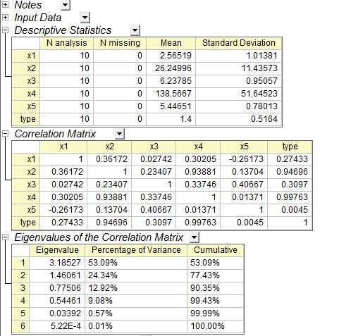
该矩阵的第三和第五列为完全随机,可以看作是所有样本都具有的共同性质,1、2、5属性则按照type值分别产生,目的是分类。
==================================================================================
因此,利用PCA进行降维分解后,理论上得到的主要主成分可以较好的分辨出两类数据;同时利用因子分析时,则可以将3和5分为一个具有共同“原因”的因子1,其他3个属性则有另外的因子2.
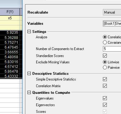
首先对矩阵进行PCA分析:
使用如下函数并显示结果如下:
> statprin = princomp(allmn[,-6])
> statprin
Call:
princomp(x = allmn[, -6])
Standard deviations:
Comp.1 Comp.2 Comp.3 Comp.4 Comp.5
50.0499858 3.6809921 1.0206695 0.8525330 0.4142678
5 variables and 10 observations.
> statprin$loadings
Loadings:
Comp.1 Comp.2 Comp.3 Comp.4 Comp.5
[1,] 0.609 -0.730 0.305
[2,] -0.205 0.973 -0.106
[3,] -0.539 -0.668 -0.510
[4,] -0.979 -0.203
[5,] -0.581 -0.146 0.797
Comp.1 Comp.2 Comp.3 Comp.4 Comp.5
SS loadings 1.0 1.0 1.0 1.0 1.0
Proportion Var 0.2 0.2 0.2 0.2 0.2
Cumulative Var 0.2 0.4 0.6 0.8 1.0
> statprin$scores
Comp.1 Comp.2 Comp.3 Comp.4 Comp.5
[1,] 34.54654 -2.413485 0.07190294 -0.34459170 0.81911670
[2,] 40.98471 -3.632566 -0.68139775 -0.12121723 -0.27943756
[3,] 41.62794 2.254175 -1.04014425 -0.47334195 -0.65073360
[4,] 39.01842 2.911636 -0.49270201 -1.26263656 0.45113400
[5,] 40.75916 -1.520744 2.55103293 0.11526931 -0.19898778
[6,] 47.75940 2.142616 -0.40017795 1.90059064 -0.07862663
[7,] -60.25960 -2.432613 -0.66973518 1.12727040 0.39856979
[8,] -60.67103 -5.976114 0.29591436 -0.52441817 -0.32806635
[9,] -63.89047 1.433254 -0.63977802 -0.37902943 -0.16410667
[10,] -59.87508 7.233839 1.00508492 -0.03789531 0.03113811
====================================================
> statprin = princomp(allmn[,-6],cor = T)
> statprin
Call:
princomp(x = allmn[, -6], cor = T)
Standard deviations:
Comp.1 Comp.2 Comp.3 Comp.4 Comp.5
1.5055210 1.2064090 0.8450579 0.7305679 0.1735850
5 variables and 10 observations.
> statprin$loadings
Loadings:
Comp.1 Comp.2 Comp.3 Comp.4 Comp.5
[1,] -0.311 0.485 0.690 0.428
[2,] -0.626 -0.332 0.148 0.686
[3,] -0.326 -0.505 0.566 -0.544 0.148
[4,] -0.626 -0.306 -0.202 -0.684
[5,] -0.115 -0.706 0.677 -0.175
Comp.1 Comp.2 Comp.3 Comp.4 Comp.5
SS loadings 1.0 1.0 1.0 1.0 1.0
Proportion Var 0.2 0.2 0.2 0.2 0.2
Cumulative Var 0.2 0.4 0.6 0.8 1.0
> statprin$scores
Comp.1 Comp.2 Comp.3 Comp.4 Comp.5
[1,] 0.9396722 -0.3130720 0.461566499 0.7029921 -0.315479156
[2,] 1.2781152 -0.8210070 0.340045316 -0.8067251 -0.002413174
[3,] 0.7353347 -1.1588953 0.535796285 -0.3944877 0.301962401
[4,] 0.2394476 -0.9836652 1.200454347 1.0634281 -0.023867354
[5,] 1.5452340 2.9524542 0.378046562 -0.2147573 -0.003596390
[6,] 2.1407842 -0.2671570 -1.665564034 0.1828104 0.108522908
[7,] -1.0721197 -0.6120581 -1.374824967 -0.1084554 -0.216636980
[8,] -1.5789550 0.4976330 0.431110498 -1.3196062 -0.110035540
[9,] -2.1464801 -0.5989192 -0.004400587 -0.1325965 0.080763513
[10,] -2.0810330 1.3046866 -0.302229919 1.0273976 0.180779771
====================================================
然后使用psych包的主成分分析得到结果如下:
默认值为:
principal(r, nfactors = 1, residuals = FALSE,rotate="varimax",n.obs=NA, covar=FALSE,
scores=TRUE,missing=FALSE,impute="median",oblique.scores=TRUE,method="regression",...)
+++++++++++++++++++++++++++++++++++
> psyprin = principal(allmn[,-6])
> psyprin
Principal Components Analysis
Call: principal(r = allmn[, -6])
Standardized loadings (pattern matrix) based upon correlation matrix
PC1 h2 u2 com
1 0.47 0.22 0.78 1
2 0.94 0.89 0.11 1
3 0.49 0.24 0.76 1
4 0.94 0.89 0.11 1
5 0.17 0.03 0.97 1
PC1
SS loadings 2.27
Proportion Var 0.45
Mean item complexity = 1
Test of the hypothesis that 1 component is sufficient.
The root mean square of the residuals (RMSR) is 0.2
with the empirical chi square 7.63 with prob < 0.18
Fit based upon off diagonal values = 0.75
> psyprin$loadings
Loadings:
PC1
[1,] 0.469
[2,] 0.942
[3,] 0.491
[4,] 0.943
[5,] 0.173
PC1
SS loadings 2.267
Proportion Var 0.453
> psyprin$residual
[,1] [,2] [,3] [,4] [,5]
[1,] 0.78028860 -0.07982963 -0.2026775 -0.13980904 -0.34276745
[2,] -0.07982963 0.11261971 -0.2283605 0.05080862 -0.02581635
[3,] -0.20267751 -0.22836055 0.7590159 -0.12530066 0.32180529
[4,] -0.13980904 0.05080862 -0.1253007 0.11137104 -0.14926199
[5,] -0.34276745 -0.02581635 0.3218053 -0.14926199 0.97011128
> psyprin$weights
PC1
[1,] 0.20680102
[2,] 0.41560547
[3,] 0.21658110
[4,] 0.41589778
[5,] 0.07627461
> psyprin$r.scores
PC1
PC1 1
> psyprin$Structure
Loadings:
PC1
[1,] 0.469
[2,] 0.942
[3,] 0.491
[4,] 0.943
[5,] 0.173
PC1
SS loadings 2.267
Proportion Var 0.453
> psyprin$scores
PC1
[1,] -0.5921215
[2,] -0.8053867
[3,] -0.4633610
[4,] -0.1508846
[5,] -0.9737079
[6,] -1.3489857
[7,] 0.6755815
[8,] 0.9949567
[9,] 1.3525749
[10,] 1.3113342
+++++++++++++++++++++++++++++++++++++++++++++++++++++++++
> psyprin = principal(allmn[,-6],nfactors = 5)
> psyprin
Principal Components Analysis
Call: principal(r = allmn[, -6], nfactors = 5)
Standardized loadings (pattern matrix) based upon correlation matrix
PC1 PC2 PC4 PC3 PC5 h2 u2 com
1 0.20 -0.14 0.01 0.97 0.00 1 3.3e-16 1.1
2 0.96 0.12 0.05 0.19 0.13 1 2.1e-15 1.2
3 0.16 0.21 0.96 0.01 0.00 1 7.8e-16 1.2
4 0.97 -0.05 0.20 0.11 -0.13 1 1.7e-15 1.2
5 0.04 0.97 0.21 -0.14 0.01 1 1.2e-15 1.1
PC1 PC2 PC4 PC3 PC5
SS loadings 1.93 1.02 1.01 1.01 0.03
Proportion Var 0.39 0.20 0.20 0.20 0.01
Cumulative Var 0.39 0.59 0.79 0.99 1.00
Proportion Explained 0.39 0.20 0.20 0.20 0.01
Cumulative Proportion 0.39 0.59 0.79 0.99 1.00
Mean item complexity = 1.1
Test of the hypothesis that 5 components are sufficient.
The root mean square of the residuals (RMSR) is 0
with the empirical chi square 0 with prob < NA
Fit based upon off diagonal values = 1
> psyprin$loadings
Loadings:
PC1 PC2 PC4 PC3 PC5
[1,] 0.197 -0.140 0.970
[2,] 0.964 0.117 0.193 0.128
[3,] 0.163 0.209 0.964
[4,] 0.965 0.196 0.106 -0.127
[5,] 0.967 0.207 -0.141
PC1 PC2 PC4 PC3 PC5
SS loadings 1.928 1.016 1.014 1.010 0.033
Proportion Var 0.386 0.203 0.203 0.202 0.007
Cumulative Var 0.386 0.589 0.791 0.993 1.000
> psyprin$residual
[,1] [,2] [,3] [,4] [,5]
[1,] 1.332268e-15 1.665335e-15 3.538836e-16 1.332268e-15 -7.771561e-16
[2,] 1.665335e-15 3.996803e-15 1.387779e-15 3.774758e-15 -4.718448e-16
[3,] 3.538836e-16 1.387779e-15 1.332268e-15 4.440892e-16 8.881784e-16
[4,] 1.332268e-15 3.774758e-15 4.440892e-16 3.774758e-15 -9.540979e-16
[5,] -7.771561e-16 -4.718448e-16 8.881784e-16 -9.540979e-16 1.110223e-15
> psyprin$weights
PC1 PC2 PC4 PC3 PC5
[1,] -0.17142891 0.175190086 -0.02602742 1.09208881 -0.5052338
[2,] 0.54668110 -0.051935582 -0.06335872 -0.12588806 3.9589214
[3,] -0.13225589 -0.241258178 1.11553425 -0.02381358 0.7973585
[4,] 0.54865918 0.009654625 -0.10930831 -0.10042751 -3.9477235
[5,] -0.03280502 1.118228274 -0.24348936 0.17302323 -0.9390233
> psyprin$r.scores
PC1 PC2 PC4 PC3 PC5
PC1 1.000000e+00 9.783840e-16 -2.879641e-16 -5.325601e-16 -1.387779e-15
PC2 9.714451e-16 1.000000e+00 -7.216450e-16 5.828671e-16 -2.220446e-15
PC4 -2.714842e-16 -7.494005e-16 1.000000e+00 -3.469447e-16 -2.942091e-15
PC3 -5.473053e-16 5.828671e-16 -3.330669e-16 1.000000e+00 -1.887379e-15
PC5 -2.715113e-16 -2.393051e-15 -2.997602e-15 -1.773321e-15 1.000000e+00
> psyprin$Structure
Loadings:
PC1 PC2 PC4 PC3 PC5
[1,] 0.197 -0.140 0.970
[2,] 0.964 0.117 0.193 0.128
[3,] 0.163 0.209 0.964
[4,] 0.965 0.196 0.106 -0.127
[5,] 0.967 0.207 -0.141
PC1 PC2 PC4 PC3 PC5
SS loadings 1.928 1.016 1.014 1.010 0.033
Proportion Var 0.386 0.203 0.203 0.202 0.007
Cumulative Var 0.386 0.589 0.791 0.993 1.000
> psyprin$scores
PC1 PC2 PC4 PC3 PC5
[1,] -0.8220315 0.8270624 -0.3656468 0.4941122 -1.65776924
[2,] -0.9140570 -0.3679674 0.8635259 -0.7644614 -0.08836774
[3,] -0.7623091 0.1487566 1.0029861 -0.4447277 1.60807138
[4,] -0.8881530 1.4965123 0.3173133 1.1093803 -0.03840412
[5,] -0.7904872 -1.9465261 -1.0964274 0.9893224 -0.04496623
[6,] -0.3632270 0.1264682 -1.5034559 -1.7256706 0.61801667
[7,] 1.2558878 0.3810522 -0.3750854 -1.1095263 -1.18221046
[8,] 0.7634519 -1.3234164 1.3439812 0.1044243 -0.72376606
[9,] 1.1500446 0.3487750 0.7971708 0.1092635 0.42907499
[10,] 1.3708807 0.3092833 -0.9843618 1.2378833 1.08032081
++++++++++++++++++++++++++++++++++++++++++++++++++++++++++++
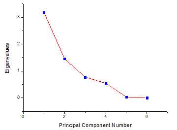
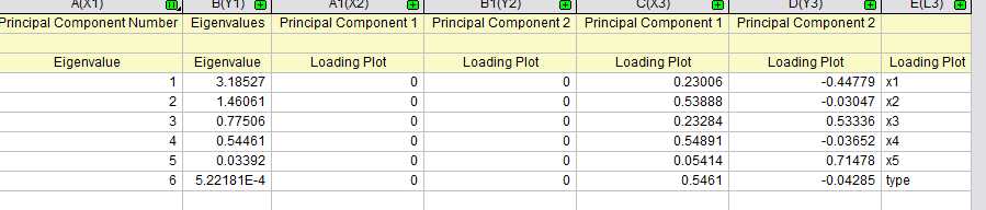
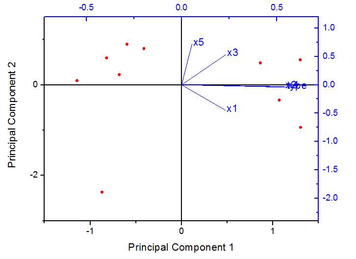
在origin中得到结果如下
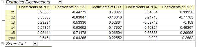
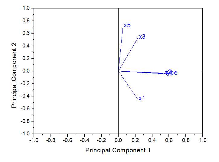
载荷图如下:
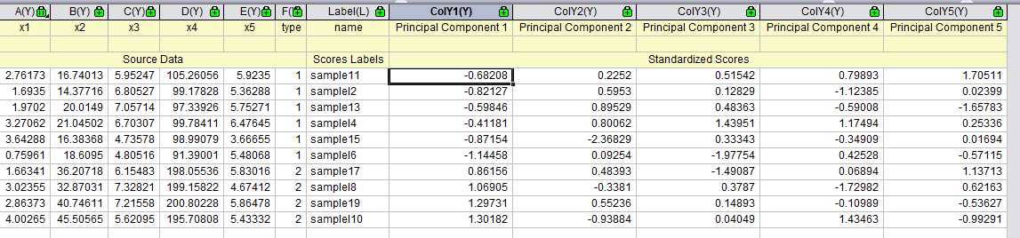
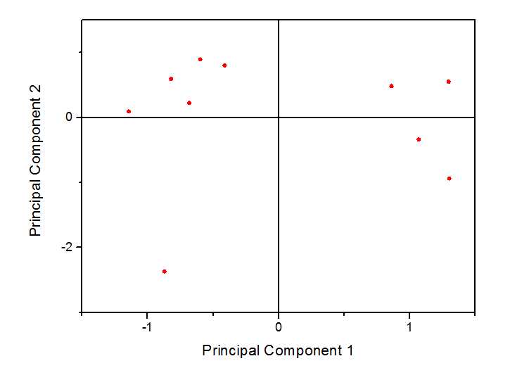
得分图如下:
双图显示:
===========================
=============================
===============================
时间不够,先上一个使用R语言也可以得到和ORIGIN软件得到的相同的结果,首先如果你要求得特征值,那么先用eigen()方法求得,并且忽略得到的特征向量,因为那个符号不一样,原因未知。同symmetric值有一点点关系,但是还不清楚是否真的有关系,该值默认为True,修改为False后有时候会有变化。
其次,你要得到正确的特征向量,需要使用prcomp()方法,注意拼写,不是principal()也不是princomp(),这几个方法是有区别的,这样你就得到了特征向量,但是没有特征值,因此加上你之前得到的特征值,你就得到了需要的特征值和特征向量,并且结果同origin得到的一样。$x值就是最后的主成分值,结果一致。
当然,根据我的试验结果,使用princomp()方法得到的结果,其特征值一致,但是特征向量和最后的主成分值的符号恰好相反,即利用origin得到的是正值,那么该函数得到的是负值。$score得到的是最后主成分的值,符号恰好相反
使用principal()方法可以使用8种旋转方式(还没有弄清楚什么意思),然后所有的结果中的$value值都是特征值,全部一致,但是特征向量都有所区别。
标签:
原文地址:http://www.cnblogs.com/arcserver/p/5442201.html