Evolutionary Computing: 5. Evolutionary Strategies

标签：

resource: Evolutionary computing, A.E.Eiben

1. What is Evolution Strategies (ES)

Evolution strategies(ES) is another member of the evolutionary algorithm family.

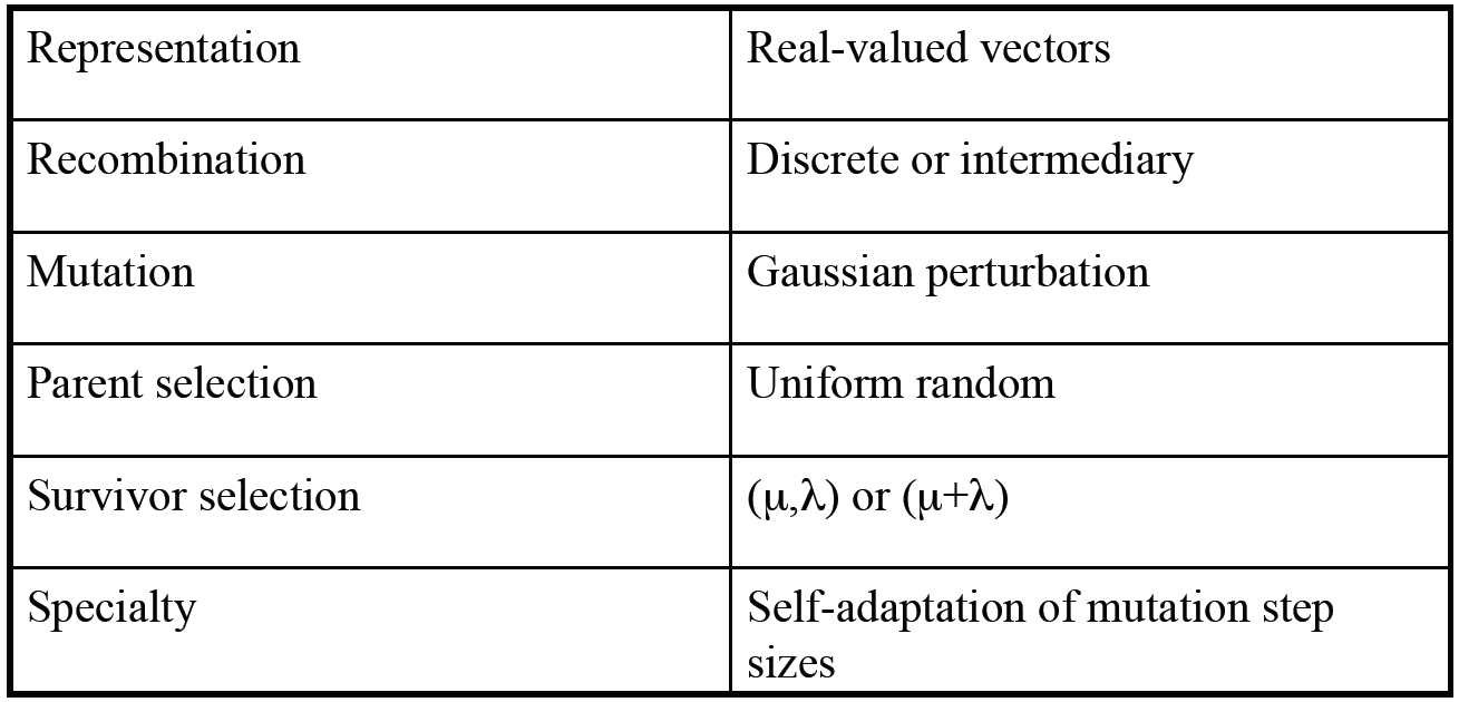
ES technical summary tableau

2. Introductory Example

2.1 Task

　　minimimise f : Rⁿ -> R 

2.2 Original algorithm

　“two-membered ES” using 

• Vectors from Rⁿ directly as chromosomes 
• Population size 1 
• Only mutation creating one child 
• Greedy selection 

2.3 pseudocde 

------------------------------------------------------------

Set t = 0

Create initial point x^t = 〈 x1^t ,…,xn^t 〉

REPEAT UNTIL (TERMIN.COND satisfied) DO

　　Draw z_i from a normal distr. for all i = 1,…,n

　　y_i^t = x_i^t + z_i

　　IF f(x^t) < f(y^t) THEN x^t+1 = x^t

　　ELSE x^t+1 = y^t

　　Set t = t+1

OD 

------------------------------------------------------------

2.4 Explanation

As is shown on the pseudocode above, given a current solution x^t in the form of a vector of length n, a new candidate x^t+1 is created by adding a random number z_i for i =1,...,n to each of the n components.

( let‘s talk about the random number Z_i )

The random number Z_i:

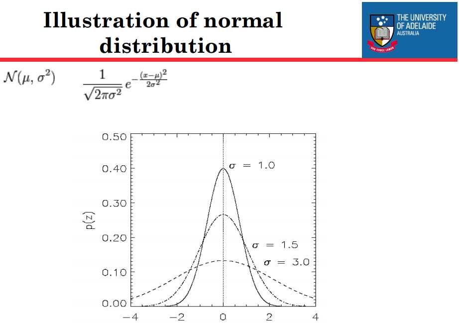
A Gaussian, or normal, distribution is used with zero mean and standard deviation σ for drawing the random numbers. 

This distribution is symmetric about zero and has the feature that the probability of drawing a random number with any given magnitude is a rapidly decreasing function of the standard deviation σ. (more information about Gaussian distribution)

( let‘s talk about the random number σ)

Thus the σ value is a parameter of the algorithm that determines the extent to which given values x_i are perturbed by the mutation operator.

For this reason σ is often called the mutation step size.  

Theoretical studies motivated an on-line adjustment of step sizes by the famous 1/5 success rule. This rule states that the ratio of successful mutaions (those in which the child is fitter than the parent) to all mutations should be 1/5.

• If the ratio is greater than 1/5, the step size should be increased to make a wider search of the space.
• If the ratio is less than 1/5 then it should be decreased to concentrate the search more around the current solution.

The rule is executed at periodic intervals.

For instance, after k iterations each σ is reset by

• σ = σ / c    if p_s > 1/5
• σ = σ • c    if p_s < 1/5
• σ = σ         if p_s = 1/5 

Where p_s is the relative frequency of successful mutations measured over a number of trials, and the parameter c is in the range [0.817,1]

As is apparent, using this mechanism the step sizes change based on feedback from the search process. 

2.5 Conclusion

This example illuminiates some essential characteristics of evolution strategies:

1. Evolution strategies are typically used for continuous parameter optimisation.
2. There is a strong emphasis on mutation for creating offspring.
3. Mutation is implemented by adding some random noise drawn from a Gaussian distribution.
4. Mutation parameters are changed during a run of the algorithm

3. Representation

Chromosomes consist of three parts: 

• Object variables: x₁,…,x_n
• Strategy parameters: 
  • Mutation step sizes: σ₁,…,σ_nσ
  • Rotation angles: α₁,…, α_nα

Full size: 〈 x₁,…,x_n, σ₁,…,σ_n ,α₁,…, α_k 〉,where k = n(n-1)/2 (no. of i,j pairs) ---This is the general form of individuals in ES

The σ values represent the mutation step sizes, and their number n_σ is usually either 1 or n. For any easonable self-adaptation mechanism at least one σ must be present.

The α values, which represent interactions between the step sizes used for different variables, are not always used.

4. Mutation

4.1 Main mechanism

Changing value by adding random noise drawn from normal distribution 

The mutation operator in ES is based on a normal (Gaussian) distribution requiring two parameters: the mean ξ and the standard deviation σ.

Mutations then are realised by adding some Δx_i to each x_i, where the Δx_i values are randomly drawn using the given Gaussian N(ξ,σ), with the corresponding probability density function.

x_i‘ = x_i + N(0,σ) 

x_i‘ can be seen as a new x_i.

N(0,σ) here denotes a random number drawn from a Gaussian distribution with zero mean and standard deviation σ.

4.2 Key ideas

•  σ is part of the chromosome 〈 x1,…,xn, σ 〉
•  σ is also mutated into σ ’ (see later how) 
• Self-adaption

4.3 A simplest case

In the simplest case we would have one step size that applied to all the components x_i and candidate solutions of the form <x₁, ..., x_n, σ>.

Mutations are then realised by replacing <x₁, ..., x_n, σ> by <x₁‘, ..., x_n‘, σ‘>, where σ‘ is the mutated value of σ and x_i‘ = x_i + N(0,σ)

4.4 Mutate the value of σ

The mutation step sizes are not set by the user; rather the σ is coevolving with the solutions.

In order to achieve this behaviour:

1. modify the value of σ first
2. mutate the x_i values with the new σ value.

The rationale behind this is that a new individual <x‘, σ‘> is effectively evaluated twice:

1. Primarily, it is evaluated directly  for its viability during survivor selection based on f(x‘).
2. Second, it is evaluated for its ability to create good offspring.

This happens indirectly: a given step size (σ) evaluates favourably if the offspring generated by using it prove viable (in the first sense).

To sum up, an individual <x‘, σ‘> represents both a good x‘ that survived selection and a good σ‘ that proved successful in generating this good x‘ from x.

4.5 Uncorrelated Mutation with One Step Size(σ)

In the case of uncorrelated mutation with one step size, the same distribution is used to mutate each x_i, therefore we only have one strategy parameter σ in each individual.

This σ is mutated each time step by multiplying it by a term e^Γ, with Γ a random variable drawn each time from a normal distribution with mean 0 and standard deviation τ.

Since N(0,τ) = τ•N(0,1), the mutation mechanism is thus specified by the following formulas:

• σ‘ = σ•e^τ•N(0,1)
• x_i‘ = x_i + σ‘•N_i(0,1) 

Furthermore, since standard deviations very close to zero are unwanted(they will have on average a negligible effect), the following boundary rule is used to force step sizes to be no smaller than a threshold:

• σ ’ < ε0 ⇒ σ ’ = ε0

Tips: 

• N(0,1) denotes a draw from the standard normal distribution
• Ni(0,1) denotes a separate draw from the standard normal distribution for each variable i.

The proportionality constant τ is an external parameter to be set by the user.

It is usually inversely proportional to the square root of the problem size:

• τ ∝ 1/ n½

The parameter τ can be interpreted as a kind of learning rate, as in neural networks.

Evolutionary Computing: 5. Evolutionary Strategies

标签：

原文地址：http://www.cnblogs.com/adelaide/p/5738878.html