标签:
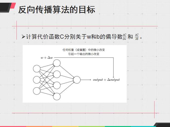
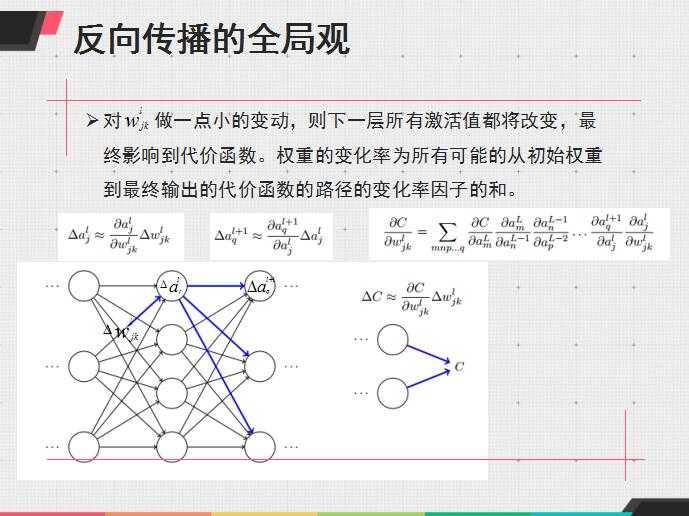
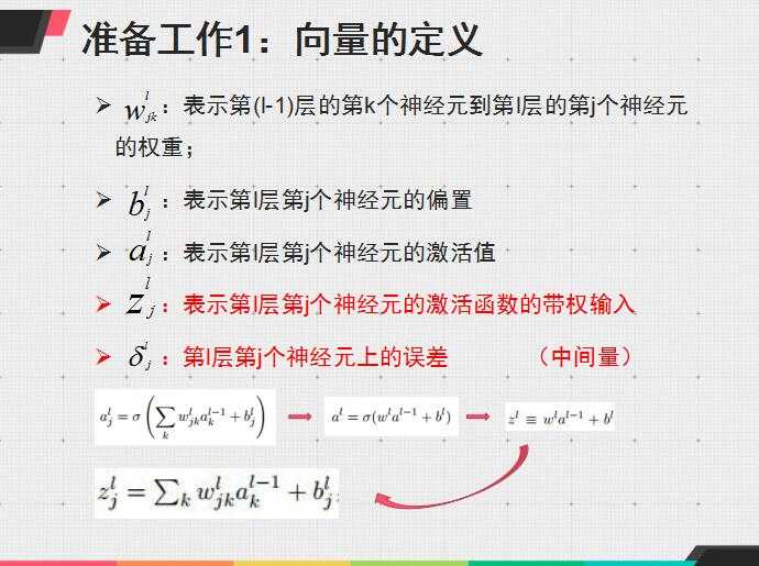
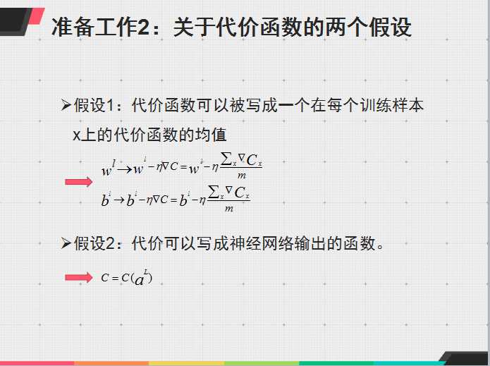
初学神经网络算法--梯度下降、反向传播、优化(交叉熵代价函数、L2规范化) 柔性最大值(softmax)还未领会其要义,之后再说
有点懒,暂时不想把算法重新总结,先贴一个之前做过的反向传播的总结ppt
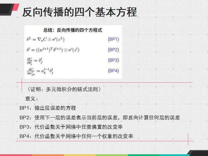

其实python更好实现些,不过我想好好学matlab,就用matlab写了
然后是算法源码,第一个啰嗦些,不过可以帮助理解算法
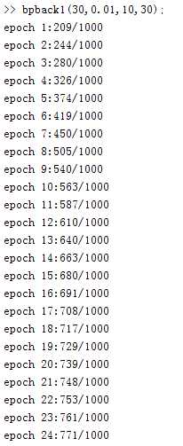
function bpback1(ny,eta,mini_size,epoch)
%ny:隐藏层为1层,神经元数目为ny;eta:学习速率;mini_size:最小采样;eopch:迭代次数
%该函数为梯度下降+反向传播
%images
[numimages,images]=bpimages(‘train-images.idx3-ubyte‘);
[n_test,test_data_x]=bpimages(‘t10k-images.idx3-ubyte‘);
%labels
[numlabels,labels]=bplabels(‘train-labels.idx1-ubyte‘);
[n_test,test_data_y]=bplabels(‘t10k-labels.idx1-ubyte‘);
%init w/b
%rand(‘state‘,sum(100*clock));
%ny=30;eta=0.01;mini_size=10;
w1=randn(ny,784);
b1=randn(ny,1);
w2=randn(10,ny);
b2=randn(10,1);
for epo=1:epoch
for nums=1:numimages/mini_size
for num=(nums-1)*mini_size+1:nums*mini_size
x=images(:,num);
y=labels(:,num);
net2=w1*x; %input of net2
for i=1:ny
hidden(i)=1/(1+exp(-net2(i)-b1(i)));%output of net2
end
net3=w2*hidden‘; %input of net3
for i=1:10
o(i)=1/(1+exp(-net3(i)-b2(i)));%output of net3
end
%back
for i=1:10
delta3(i)=(y(i)-o(i))*o(i)*(1-o(i));%delta of net3
end
for i=1:ny
delta2(i)=delta3*w2(:,i)*hidden(i)*(1-hidden(i));%delta of net2
end
%updata w/b
for i=1:10
for j=1:ny
w2(i,j)=w2(i,j)+eta*delta3(i)*hidden(j)/mini_size;
end
end
for i=1:ny
for j=1:784
w1(i,j)=w1(i,j)+eta*delta2(i)*x(j)/mini_size;
end
end
for i=1:10
b2(i)=b2(i)+eta*delta3(i);
end
for i=1:ny
b1(i)=b1(i)+eta*delta2(i);
end
end
end
%calculate sum of error
%accuracy
sum0=0;
for i=1:1000
x0=test_data_x(:,i);
y0=test_data_y(:,i);
a1=[];
a2=[];
s1=w1*x0;
for j=1:ny
a1(j)=1/(1+exp(-s1(j)-b1(j)));
end
s2=w2*a1‘;
for j=1:10
a2(j)=1/(1+exp(-s2(j)-b2(j)));
end
a2=a2‘;
[m1,n1]=max(a2);
[m2,n2]=max(y0);
if n1==n2
sum0=sum0+1;
end
%e=o‘-y;
%sigma(num)=e‘*e;
sigma(i)=sumsqr(a2-y0); %代价为误差平方和
end
sigmas(epo)=sum(sigma)/(2*1000);
fprintf(‘epoch %d:%d/%d\n‘,epo,sum0,1000);
end
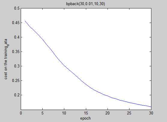
plot(sigmas);
xlabel(‘epoch‘);
ylabel(‘cost on the training_data‘);
end
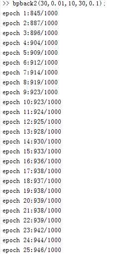
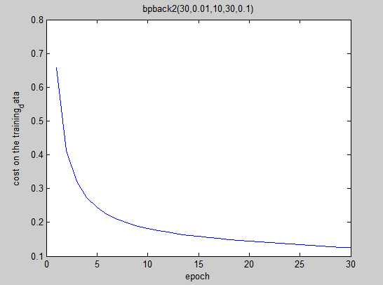
function bpback2(ny,eta,mini_size,epoch,numda)
%ny:隐藏层为1层,神经元数目为ny;eta:学习速率;mini_size:最小采样;eopch:迭代次数
%bpback的优化,包括L2规范化、交叉熵代价函数的引入---结果证明该优化非常赞!
%images
[numimages,images]=bpimages(‘train-images.idx3-ubyte‘);
[n_test,test_data_x]=bpimages(‘t10k-images.idx3-ubyte‘);
%labels
[numlabels,labels]=bplabels(‘train-labels.idx1-ubyte‘);
[n_test,test_data_y]=bplabels(‘t10k-labels.idx1-ubyte‘);
%init w/b
%ny=30;eta=0.05;mini_size=10;epoch=10;numda=0.1;
rand(‘state‘,sum(100*clock));
w1=randn(ny,784)/sqrt(784);
b1=randn(ny,1);
w2=randn(10,ny)/sqrt(ny);
b2=randn(10,1);
for epo=1:epoch
for nums=1:numimages/mini_size
    for num=(nums-1)*mini_size+1:nums*mini_size
        x=images(:,num);
        y=labels(:,num);
    net2=w1*x;               %input of net2
    hidden=1./(1+exp(-net2-b1));%output of net2
    net3=w2*hidden;            %input of net3
    o=1./(1+exp(-net3-b2));%output of net3
    %back
    delta3=(y-o);%delta of net3   由于交叉熵代价函数的引入,偏导被消去
    delta2=w2‘*delta3.*(hidden.*(1-hidden));%delta of net2
    %updata w/b
    w2=w2*(1-eta*numda/numimages)+eta*delta3*hidden‘/mini_size;     %L2规范化
    w1=w1*(1-eta*numda/numimages)+eta*delta2*x‘/mini_size;
    b2=b2+eta*delta3/mini_size;
    b1=b1+eta*delta2/mini_size;
    end
end
%calculate sum of error
%accuracy
sum0=0;
for i=1:1000
    x0=test_data_x(:,i);
    y0=test_data_y(:,i);
    a1=[];
    a2=[];
    a1=1./(1+exp(-w1*x0-b1));
    a2=1./(1+exp(-w2*a1-b2));
    [m1,n1]=max(a2);
    [m2,n2]=max(y0);
    if n1==n2
        sum0=sum0+1;
    end
    %e=o‘-y;
    %sigma(num)=e‘*e;
    sigma(i)=m2*log(m1)+(1-m2)*log(1-m1);   %计算代价cost
end
sigmas(epo)=-sum(sigma)/1000;       %cost求和
fprintf(‘epoch %d:%d/%d\n‘,epo,sum0,1000);
end
plot(sigmas);
xlabel(‘epoch‘);
ylabel(‘cost on the training_data‘);
end
好好学习,天天向上,话说都没有表情用,果然是程序猿的世界,我还是贴个表情吧

标签:
原文地址:http://www.cnblogs.com/fanmu/p/5926087.html