标签:att card receiver complete who ecif nts cto his
The linear regression model discussed in Chapter 3 assumes that the response variable Y is quantitative. But in many situations, the response variable is instead qualitative.
In this chapter we discuss three of the most widely-used classifiers: logistic regression, linear discriminant analysis, and K-nearest neighbors. We discuss more computer-intensive methods in later chapters, such as generalized additive models (Chapter 7), trees, random forests, and boosting (Chapter 8), and support vector machines (Chapter 9).
4.3 Logistic Regression
4.3.1 The Logistic Model
logistic function:
$$p(X) = \frac{e^{\beta_0+\beta_1X}}{1+e^{\beta_0+\beta_1X}} (4.2) $$
where, $p(X) = Pr(Y=1|X)$
log-odds, or logit:
$$log(\frac{p(X)}{1-p(X)}) = \beta_0 + \beta_1X$$
4.3.2 Estimating the Regression Coefficients
maximum likelihood method: we try to find $\hat{β}_0$ and $\hat{β}_1$ such that plugging these estimates into the model for p(X), given in (4.2), yields a number close to one for all individuals who defaulted, and a number close to zero for all individuals who did not.
likelihood function:
$$l(\beta_0, \beta_1) = \prod _{i:y_i=1}p(x_i)+\prod _{i‘:y_{i‘}=0}(1-p(x_{i‘}))$$
4.3.3 Making Predictions
Once the coefficients have been estimated, it is a simple matter to compute the probability of default for any given credit card balance by using the formula
$$p(X) = \frac{e^{\beta_0+\beta_1X}}{1+e^{\beta_0+\beta_1X}}$$
4.3.4 Multiple Logistic Regression
we can generalize the functions as
$$p(X) = \frac{e^{\beta_0+\beta_1X+...+\beta_pX_p}}{1+e^{\beta_0+\beta_1X+...+\beta_pX_p}}$$
$$log(\frac{p(X)}{1-p(X)}) = \beta_0 + \beta_1X+...+\beta_pX_p$$
4.4 Linear Discriminant Analysis
Why do we need another method, when we have logistic regression? There are several reasons:
4.4.1 Using Bayes’ Theorem for Classification
Let $\pi_k$ represent the overall or prior probability that a randomly chosen observation comes from the kth class; this is the probability that a given observation is associated with the kth category of the response variable Y . Let $f_k(X) ≡ Pr(X = x|Y = k)$ denote the density function of X for an observation that comes from the kth class. Then Bayes‘ theorem states that
$$p_k(X) = Pr(Y=k|X=x) =\frac{ \pi_kf_k(x)}{\sum^{K}_{l=1}\pi_lf_l(x)}$$
We refer to $p_k(x)$ as the posterior probability that an observation X = x belongs to the kth class. That is, it is the probability that the observation belongs to the kth class, given the predictor value for that observation.
4.4.2 Linear Discriminant Analysis for p = 1
The linear discriminant analysis (LDA) method approximates the Bayes classifier by plugging estimates for $π_k$, $μ_k$, and $σ^2$ into
![]()
assign an observation X = x to the class for which $\hat \delta_k(x)$ is largest.
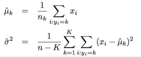
In particular, the following estimates are used:
![]()
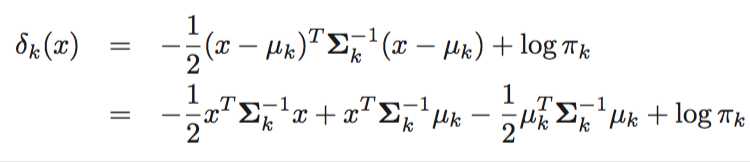
4.4.3 Linear Discriminant Analysis for p > 1
Once again, we need to estimate the unknown parameters $μ_1,...,μ_K, π_1,...,π_K$, and $Σ$; the formulas are similar to those used in the one-dimensional case. To assign a new observation X = x, LDA plugs these estimates into (4.19) and classifies to the class for which $\hat \delta_k(x)$ is largest.
![]() (4.19)
(4.19)
A binary classifier such as this one can make two types of errors
A confusion matrix is a convenient way to display this information
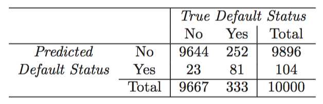
A credit card company might particularly wish to avoid incorrectly classifying an individual who will default.
In the two-class case, this amounts to assigning an observation to the default class if $Pr(default = Yes|X = x)>0.5$
Instead, we could make the threshhold as $Pr(default = Yes|X = x)>0.2$
The ROC curve is a popular graphic for simultaneously displaying the two types of errors for all possible thresholds. It is an acronym for receiver operating characteristics.
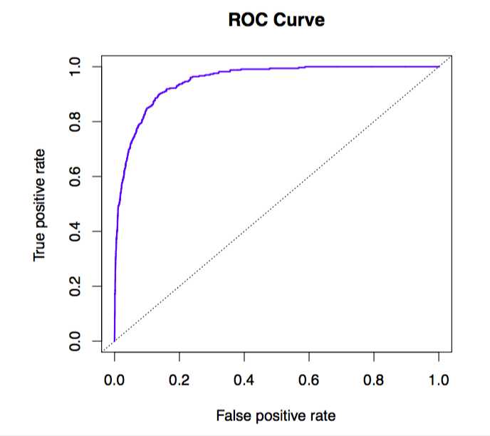
The true positive rate is the sensitivity: the fraction of defaulters that are correctly identified, using a given threshold value. The false positive rate is 1-specificity: the fraction of non-defaulters that we classify incorrectly as defaulters, using that same threshold value. The ideal ROC curve hugs the top left corner, indicating a high true positive rate and a low false positive rate. The dotted line represents the “no information” classifier; this is what we would expect if student status and credit card balance are not associated with probability of default.
4.4.4 Quadratic Discriminant Analysis (QDA)
Unlike LDA, QDA assumes that each class has its own covariance matrix. That is, it assumes that an observation from the kth class is of the form X ~ N(μk,Σk), where Σk is a covariance matrix for the kth class.
Bias-variance trade-off: roughly speaking, LDA tends to be a better bet than QDA if there are relatively few training observations and so reducing variance is crucial.
4.5 A Comparison of Classification Methods
In sum, when the true decision boundaries are linear, then the LDA and logistic regression approaches will tend to perform well. When the boundaries are moderately non-linear, QDA may give better results. Finally, for much more complicated decision boundaries, a non-parametric approach such as KNN can be superior. But the level of smoothness for a non-parametric approach must be chosen carefully.
标签:att card receiver complete who ecif nts cto his
原文地址:http://www.cnblogs.com/sheepshaker/p/6654075.html