标签:最好 创建 product red component gauss 带宽 eset 技术
学习利用sklearn的几个聚类方法:
一.几种聚类方法
1.高斯混合聚类(mixture of gaussians)
2.k均值聚类(kmeans)
3.密度聚类,均值漂移(mean shift)
4.层次聚类或连接聚类(ward最小离差平方和)
二.评估方法
1.完整性:值:0-1,同一个类别所有数据样本是否划分到同一个簇中
2.同质性:值:0-1,每个簇是否只包含同一个类别的样本
3.上面两个的调和均值
4.以上三种在评分时需要用到数据样本的真正标签,但实际很难做到。轮廓系数(1,-1):只使用聚类的数据,它计算的是每个数据样本与同簇数据样本和其它簇数据样本之间的相似度,因为从平均来看,与同簇比较起来,比其它簇更相似。
三.说明
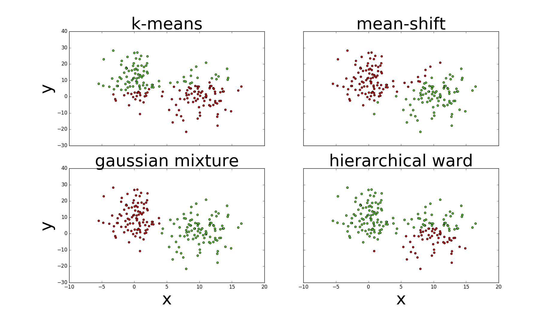
1.kmeans与高斯需要指定簇的数量(n_clusters=2,n_components=2);均值漂移指定带宽(bandwidth=7);层次使用ward链接定义合并代价(距离),终止最大距离max_d。
2.图中可以看出高斯的评估指标最好,其次是均值漂移,k均值与层次较差
四.sklearn聚类
  1 #!/usr/bin/python
  2 # -*- coding: utf-8 -*-
  3
  4 import numpy as np
  5 import matplotlib.pyplot as plt
  6 from sklearn.cluster import KMeans
  7 from sklearn.cluster import MeanShift
  8 from sklearn.metrics import homogeneity_completeness_v_measure
  9 from sklearn import mixture
 10 from scipy.cluster.hierarchy import linkage
 11 from scipy.cluster.hierarchy import fcluster
 12
 13 class ClusterMethod:
 14
 15     def __init__(self):
 16         l1=np.zeros(100)
 17         l2=np.ones(100)
 18         self.labels=np.concatenate((l1,l2),)
 19
 20     #随机创建两个二维正太分布,形成数据集
 21     def dataProduction(self):
 22         # 随机创建两个二维正太分布,形成数据集
 23         np.random.seed(4711)
 24         c1 = np.random.multivariate_normal([10, 0], [[3, 1], [1, 4]], size=[100, ])
 25         l1 = np.zeros(100)
 26         l2 = np.ones(100)
 27         # 一个100行的服从正态分布的二维数组
 28         c2 = np.random.multivariate_normal([0, 10], [[3, 1], [1, 4]], size=[100, ])
 29         # 加上一些噪音
 30         np.random.seed(1)
 31         noise1x = np.random.normal(0, 2, 100)
 32         noise1y = np.random.normal(0, 8, 100)
 33         noise2 = np.random.normal(0, 8, 100)
 34         c1[:, 0] += noise1x  # 第0列加入噪音数据
 35         c1[:, 1] += noise1y
 36         c2[:, 1] += noise2
 37
 38         # 定义绘图
 39         self.fig = plt.figure(figsize=(20, 15))
 40         # 添加子图,返回Axes实例,参数:子图总行数,子图总列数,子图位置
 41         ax = self.fig.add_subplot(111)
 42         # x轴
 43         ax.set_xlabel(‘x‘, fontsize=30)
 44         # y轴
 45         ax.set_ylabel(‘y‘, fontsize=30)
 46         # 标题
 47         self.fig.suptitle(‘classes‘, fontsize=30)
 48         # 连接
 49         labels = np.concatenate((l1, l2), )
 50         X = np.concatenate((c1, c2), )
 51         # 散点图
 52         pp1 = ax.scatter(c1[:, 0], c1[:, 1], cmap=‘prism‘, s=50, color=‘r‘)
 53         pp2 = ax.scatter(c2[:, 0], c2[:, 1], cmap=‘prism‘, s=50, color=‘g‘)
 54         ax.legend((pp1, pp2), (‘class 1‘, ‘class 2‘), fontsize=35)
 55         self.fig.savefig(‘scatter.png‘)
 56         return X
 57
 58     def clusterMethods(self):
 59         X=self.dataProduction()
 60         self.fig.clf()#reset plt
 61         self.fig,((axis1,axis2),(axis3,axis4))=plt.subplots(2,2,sharex=‘col‘,sharey=‘row‘)#函数返回一个figure图像和一个子图ax的array列表
 62
 63         #k-means
 64         self.kMeans(X,axis1)
 65         #mean-shift
 66         self.meanShift(X,axis2)
 67         #gaussianMix
 68         self.gaussianMix(X,axis3)
 69         #hierarchicalWard
 70         self.hierarchicalWard(X,axis4)
 71
 72     def kMeans(self,X,axis1):
 73         kmeans=KMeans(n_clusters=2)#聚类个数
 74         kmeans.fit(X)#训练
 75         pred_kmeans=kmeans.labels_#每个样本所属的类
 76         print(‘kmeans:‘,np.unique(kmeans.labels_))
 77         print(‘kmeans:‘,homogeneity_completeness_v_measure(self.labels,pred_kmeans))#评估方法,同质性,完整性,两者的调和平均
 78         #plt.scatter(X[:,0],X[:,1],c=kmeans.labels_,cmap=‘prism‘)
 79         axis1.scatter(X[:,0],X[:,1],c=kmeans.labels_,cmap=‘prism‘)
 80         axis1.set_ylabel(‘y‘,fontsize=40)
 81         axis1.set_title(‘k-means‘,fontsize=40)
 82         #plt.show()
 83
 84     def meanShift(self,X,axis2):
 85         ms=MeanShift(bandwidth=7)#带宽
 86         ms.fit(X)
 87         pred_ms=ms.labels_
 88         axis2.scatter(X[:,0],X[:,1],c=pred_ms,cmap=‘prism‘)
 89         axis2.set_title(‘mean-shift‘,fontsize=40)
 90         print(‘mean-shift:‘,np.unique(ms.labels_))
 91         print(‘mean-shift:‘,homogeneity_completeness_v_measure(self.labels,pred_ms))
 92
 93     def gaussianMix(self,X,axis3):
 94         gmm=mixture.GMM(n_components=2)
 95         gmm.fit(X)
 96         pred_gmm=gmm.predict(X)
 97         axis3.scatter(X[:, 0], X[:, 1], c=pred_gmm, cmap=‘prism‘)
 98         axis3.set_xlabel(‘x‘, fontsize=40)
 99         axis3.set_ylabel(‘y‘, fontsize=40)
100         axis3.set_title(‘gaussian mixture‘, fontsize=40)
101         print(‘gmm:‘,np.unique(pred_gmm))
102         print(‘gmm:‘,homogeneity_completeness_v_measure(self.labels,pred_gmm))
103
104     def hierarchicalWard(self,X,axis4):
105         ward=linkage(X,‘ward‘)#训练
106         max_d=110#终止层次算法最大的连接距离
107         pred_h=fcluster(ward,max_d,criterion=‘distance‘)#预测属于哪个类
108         axis4.scatter(X[:,0], X[:,1], c=pred_h, cmap=‘prism‘)
109         axis4.set_xlabel(‘x‘,fontsize=40)
110         axis4.set_title(‘hierarchical ward‘,fontsize=40)
111         print(‘ward:‘,np.unique(pred_h))
112         print(‘ward:‘,homogeneity_completeness_v_measure(self.labels,pred_h))
113
114         self.fig.set_size_inches(18.5,10.5)
115         self.fig.savefig(‘comp_clustering.png‘,dpi=100)#保存图
116
117 if __name__==‘__main__‘:
118     cluster=ClusterMethod()
119     cluster.clusterMethods()
五.评估图
参考:1.Machine.Learning.An.Algorithmic.Perspective.2nd.Edition.
2.Machine Learning for the Web
标签:最好 创建 product red component gauss 带宽 eset 技术
原文地址:http://www.cnblogs.com/little-horse/p/7367407.html