摘自:http://davis.wpi.edu/~matt/courses/clipping/
| Motivation |
Motivation
Clipping is an essential part of image synthesis. Traditionally, polygon clipping has been used to clip out the portions of a polygon that lie outside the window of the output device to prevent undesirable effects. In the recent past polygon clipping is used to render 3D images through hidden surface removal and to produce high-quality surface details using techniques such as Beam tracing. Polygon clipping is also used in distributing the objects of a scene to appropriate processors in multiprocessor raytracing systems to improve rendering speeds.
Clipping an arbitrary polygon against an arbitrary polygon is a basic routine in computer graphics. In rendering complex images, it may be applied thousands of times. The efficiency of these routines is therefore extremely important. To achieve good results, most of the commercial products use simplified clipping algorithms that can only clip regular (e.g. convex) polygons. However, due to the development of new products that require complex modelling of the objects (e.g. CAD applications) the need of finding efficient methods for clipping more general polygons (e.g. concave or self-intersecting polygons) has become stringent. So far though, only two other algorithms have been proposed. In 1980, Weiler designed for the first time an algorithms which was able to clip arbitrary polygons. His approach was based on a graph representation of the polygons and was rather complicated. In order to generate the result polygon, a complete traversal of a tree structure was necessary. Only 12 year later, Vatti proposed a new algorithm. His method was able to perform some other boolean operations on the two input polygons and offered support to an eventual further filling process. However, the data structure they use was more complex that in the algorithm presented. Moreover, the intersection between the cross intersecting edges of a polygon has also to be computed. This leads to poorer results in comparison with the present algorithm.
Definitions. A closed polygon is defined as an ordered list of nodes in which the first and the last one (and possible others too) are identical. Further, given two polygons - a clip (clipper) and a subject polygon (cleppee) - the clipped polygon is defines as the set of all points interior to the clip polygon that lie inside the subject polygon. This set will be either a single polygon or a set of new polygons.
But what does "interior" mean for a self-intersecting polygon? In order to define a containment criterion, the "winding number" has been introduced. Intuitively, the winding number of a point A shows how many times a ray originated in A winds around A when moving along a close curve w. Formally, the winding number is defined as an integral:

where the variable to be integrated in a positive angle obtained by moving the ray along the curve:
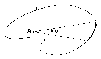
Now, we can define the interior of a curve w as the set of points for which the winding number is odd:
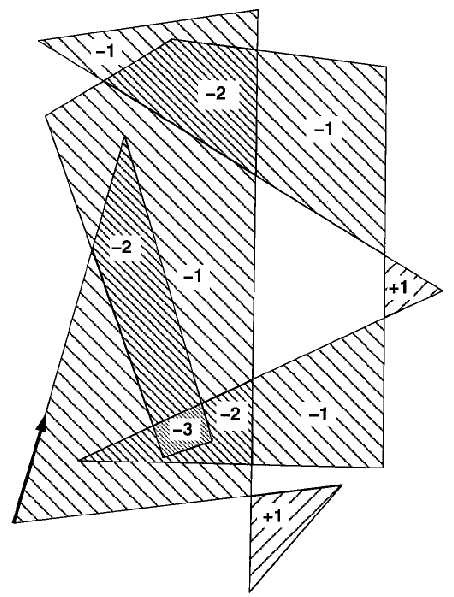
The winding numbers have some important properties, such as:
the winding number remains constant when the point (A) or the curve (w) change, as long as A keeps a positive distance to w;
the components of the subspace RxR - w have the same winding number; specifically, the winding numbers for the points situated in unbounded regions is zero.
by crossing the curve, the winding number changes by exactly 1 (+/-1).
These properties give an efficient way to compute the interior test. The testing method, based on a line scan of the polygon is presented in [2]. The idea is that, coming from infinity (where the winding number is zero) a ray changes is inside / outside status every time it
intersects an edge.
The algorithm computes the clipped polygon in three phases. In the first phase it determines (and marks) the intersection points. The points are then inserted in both lists, in their proper place by ordering them using the alpha values. If no intersection points are found in this phase we know that either the subject polygon lies entirely inside the clip polygon or vice versa, or that both polygons are disjoint. By performing a containment test for any of the vertexes we are able to determine which case we have. Then we either return the inner polygon or nothing at all.
In order to efficiently implement this, the algorithm uses two doubly linked lists to represent the polygons. One list is for the clip and one for the subject polygon. In each list, a node represents a distinct vertex. Obviously, the lists will contain the x and y coordinates of the vertexes as well as the necessary links to the previous and next node in the list. In addition to these however, the algorithm needs some more information:
typedef struct _node
{
int x, y;
struct _node *next;
struct _node *prev;
struct _node *nextPoly; /* pointer to the next polygon */
struct _node *neighbor; /* the corresponding intersection point */
int intersect; /* 1 if an intersection point, 0 otherwise */
int entry; /* 1 if an entry point, 0 otherwise */
int visited; /* 1 if the node has been visited, 0 otherwise */
float alpha; /* intersection point placemet */
} node;
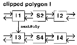
NextPoly is a pointer to a new polygon, once the current one has been closed. Indeed, in the most general case, the result of the algorithm is a set of polygons rather than a single one, so that the lists that represent the polygons have to be linked together in order for polygons to be accessed from one to another.
Intersect is a boolean value that is set to true if the current node is an intersection point and to false otherwise. Similarly, entry is flag that records whether the intersecting point is an entry or an exit point to the other polygon‘s interior.
Neighbor is a link to the identical vertex in the "neighbor" list. An intersection node belongs, obviously, to both polygons and therefore has to be present in both lists of vertexes. However, in Phase III, when we generate the polygons from the list of resulting edges we want to be able to jump from one polygon to another (switch the current polygon). To enable that, the neighbor pointers keep track of the
identical vertexes. In the same phase of building the polygons by navigating through the list of nodes, the visited flag is used to mark the nodes already inserted in the result (it is important to notice here that every intersection point belongs to the resulting polygon (since by definition it belongs to both interiors).
The alpha value is a floating point number from 0 to 1 that indicates the position of an intersection point reported to two consecutive
non-intersection vertexes from the initial list of vertexes.
Phase one. The first phase is basically an iteration through the both lists (the complexity is at least m*n, where m and n are the number of vertexes for the two polygons). The intersection points between all the edges are determined. An important thing to remark is that here, unlike in the Vatti‘s algorithm, only the intersection points between edges from different polygons are considered.
Once a new intersection point is determined, it is inserted in both the two lists. A link between these nodes is maintain through the "neighbor" value. These links will further be used in the navigation process describe in phase three. While computing an intersection point, the algorithm determines also its alpha value. The alpha value shows basically the placement of the intersection point between the two polygon vertexes. If the length of the new formed segment is a and the length of the edge it belongs to is b, then the alpha value is defined as a/b (the value is obviously between 0 and 1). Alpha is used when inserting the new intersection points. They basically define an ordering relation on the number of intersection points between the two vertexes of the same edge.
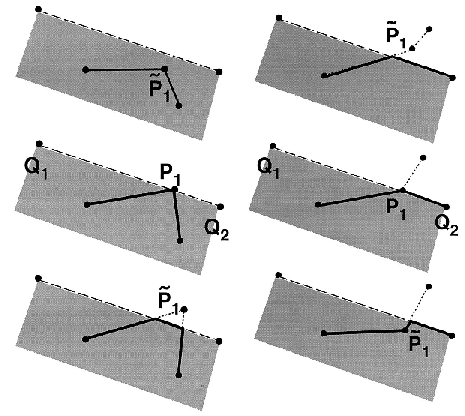
This phase of the algorithm is the most time consuming one. Determining the intersection requires floating points operations and floating points operation are computationally expensive. Moreover, we can have many degeneration cases which unfortunately increase the computation time. These problems have been solved by perturbing the "problem nodes" a method that is usually faster than addressing all the exception rules. The two perturbation choices (methods) for the two major cases of degenerating are shown below:
Phase two. Phase two is a simple process of marking the intersection points as entries or exits. Practically, the intersection points are labeled as entry/exit alternatively when traversing the polygon lists, since we cannot have two entry/exit points in a row. The process starts by first determining the inside/outside value for one vertex of each of the polygons. If, for example, it is outside the other
polygon, then the next intersection point that come across will be marked as entry. What it is interesting here is that, by changing the order in which one starts marking the nodes, other boolean operations on the set of polygons (specifically union and difference) can also be performed.
Consequently, the only problem in this phase is finding a "containment test" that, given a point and a polygon, determines whether the point lies inside that polygon or not. However, based on the observations in Section 1 (the properties of the winding numbers), a quick method can be found ([2]).
Phase three. The goal of phase three is to generate the clipped polygon (set of polygons). The generation process is a back and forth navigation through the two lists, guided by the entry/exit values and the neighbor pointers. The generation of a single polygon starts at
an intersection point. If the point is an entry then go forward till the next intersection point is reached (otherwise go backward). From this point switch the list by using the neighbor link. Further go forward or backward depending on whether the "neighbor" vertex is an entry or an exit. This process iterates until the starting point is reached, when we complete the generation of the polygon. In case that there still are unvisited nodes (every node is marked as visited or not) then the result is composed by multiple polygons and a new iteration begins.
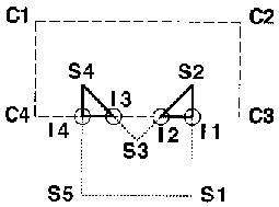
The execution of the algorithm for a small example is illustrated below:
 |  |
 |
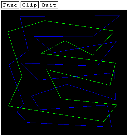
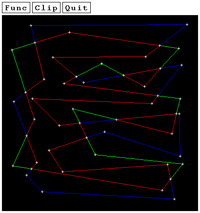
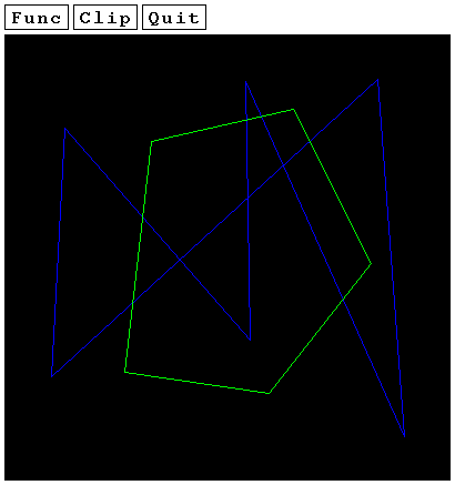
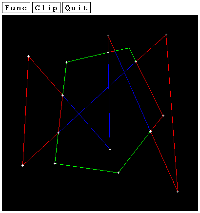
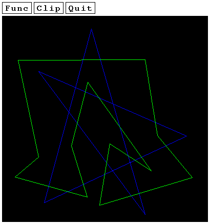
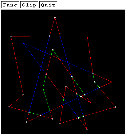
I have implemented the algorithm in C, using as a front-end tool the graphical package libsx. The user can define arbitrary polygons by simply clicking with the mouse in the drawing area and then can specify the desired functionality (intersection, union, difference) by selecting an option in the drill-down menu (the default setting is intersection). A complete version of the implementation can be found here. Below, there are some screen previews illustrating the execution window for the three typical cases. First we have the intersection of the subject (blue) polygon and the clip (green) polygon, then the difference and finally the union. Notice that union can lead to interesting results when applied to self-intersecting polygons.
 |  |
 |  |
 |  |
The algorithm presented here as well as the Vatti‘s one [3] have been implemented and compared. The tests have been performed on a SGI Indigo work station.
The method they used assumed that both the clip and the subject polygons had the same number of nodes n. For that number, one thousand polygons were randomly generated. The computation time was then averaged. The test results are presented below:

The improvement over the previous approach is obvious. The authors explain this by the fact that Vetti‘s algorithm needs also to compute the intersection points for the self-intersecting polygons. The number of such self-intersections could be quadratic in the worst case.
Some of the figures used in this presentation have been obtained from [1]. The title photography has been provided by photo.net.
原文地址:http://fengyuzaitu.blog.51cto.com/5218690/1972935