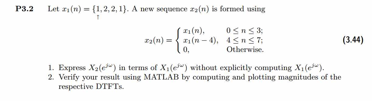
1、用x1序列的DTFT来表示x2序列的DTFT
2、代码:
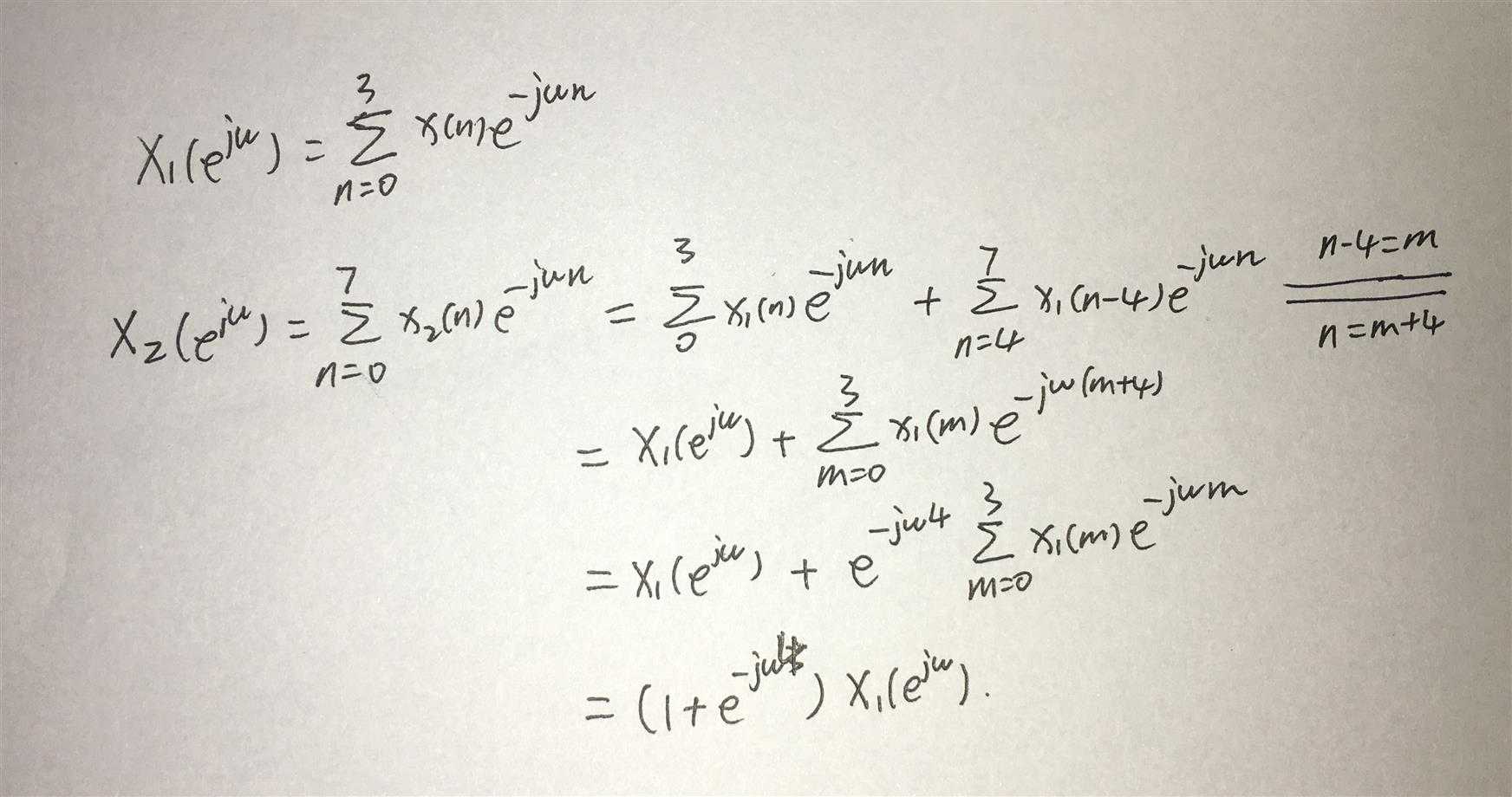
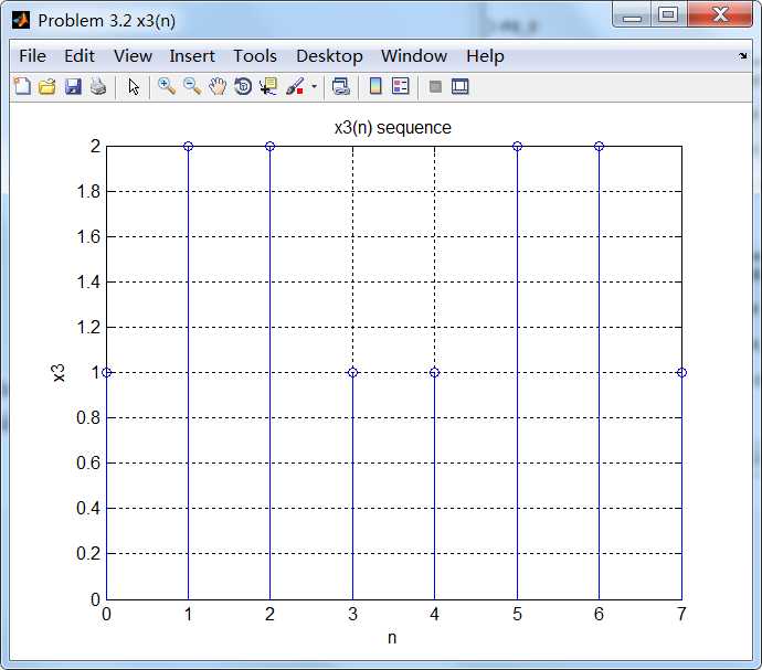
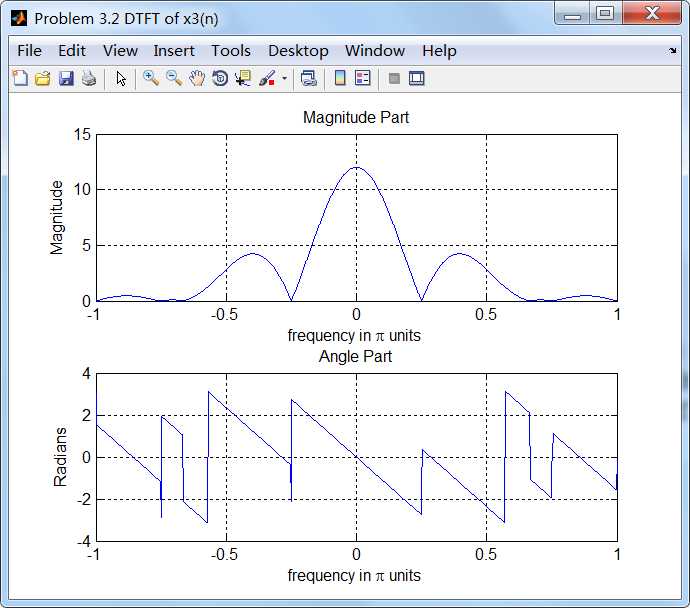
%% ------------------------------------------------------------------------
%%            Output Info about this m-file
fprintf(‘\n***********************************************************\n‘);
fprintf(‘        <DSP using MATLAB> Problem 3.2 \n\n‘);

banner();
%% ------------------------------------------------------------------------


% ----------------------------------
%            x1(n)
% ----------------------------------
n1_start = 0; n1_end = 3;
n1 = [n1_start : n1_end];

x1 = [1, 2, 2, 1];

figure(‘NumberTitle‘, ‘off‘, ‘Name‘, ‘Problem 3.2 x1(n)‘);
set(gcf,‘Color‘,‘white‘);
stem(n1, x1);
xlabel(‘n‘); ylabel(‘x1‘);
title(‘x1(n) sequence‘); grid on;

M = 500;
k = [-M:M];        % [-pi, pi]
%k = [0:M];        % [0, pi]
w = (pi/M) * k;

[X1] = dtft(x1, n1, w);

magX1 = abs(X1); angX1 = angle(X1); realX1 = real(X1); imagX1 = imag(X1);

figure(‘NumberTitle‘, ‘off‘, ‘Name‘, ‘Problem 3.2 DTFT of x1(n)‘);;
set(gcf,‘Color‘,‘white‘);
subplot(2,1,1); plot(w/pi, magX1); grid on;
title(‘Magnitude Part‘);
xlabel(‘frequency in \pi units‘); ylabel(‘Magnitude‘);
subplot(2,1,2); plot(w/pi, angX1); grid on;
title(‘Angle Part‘);
xlabel(‘frequency in \pi units‘); ylabel(‘Radians‘);


X1_chk = (1+exp(-j*w*4)) .* X1;
magX1_chk = abs(X1_chk); angX1_chk = angle(X1_chk); realX1_chk = real(X1_chk); imagX1_chk = imag(X1_chk);

figure(‘NumberTitle‘, ‘off‘, ‘Name‘, ‘Problem 3.2 X2(w) obtained by formular with X1(w)‘);;
set(gcf,‘Color‘,‘white‘);
subplot(2,1,1); plot(w/pi, magX1_chk); grid on;
title(‘Magnitude Part‘);
xlabel(‘frequency in \pi units‘); ylabel(‘Magnitude‘);
subplot(2,1,2); plot(w/pi, angX1_chk); grid on;
title(‘Angle Part‘);
xlabel(‘frequency in \pi units‘); ylabel(‘Radians‘);


% -------------------------------------
%            x2(n)
% -------------------------------------
[x2, n2] = sigshift(x1, n1, 4);


figure(‘NumberTitle‘, ‘off‘, ‘Name‘, ‘Problem 3.2 x2(n)‘);
set(gcf,‘Color‘,‘white‘);
stem(n2, x2);
xlabel(‘n‘); ylabel(‘x2‘);
title(‘x2(n) sequence‘); grid on;


M = 500;
k = [-M:M];        % [-pi, pi]
%k = [0:M];        % [0, pi]
w = (pi/M) * k;

[X2] = dtft(x2, n2, w);

magX2 = abs(X2); angX2 = angle(X2); realX2 = real(X2); imagX2 = imag(X2);

figure(‘NumberTitle‘, ‘off‘, ‘Name‘, ‘Problem 3.2 DTFT of x2(n)‘);;
set(gcf,‘Color‘,‘white‘);
subplot(2,1,1); plot(w/pi, magX2); grid on;
title(‘Magnitude Part‘);
xlabel(‘frequency in \pi units‘); ylabel(‘Magnitude‘);
subplot(2,1,2); plot(w/pi, angX2); grid on;
title(‘Angle Part‘);
xlabel(‘frequency in \pi units‘); ylabel(‘Radians‘);


% -------------------------------------
%            x3(n)
% -------------------------------------
[x3, n3] = sigadd(x1, n1, x2, n2);


figure(‘NumberTitle‘, ‘off‘, ‘Name‘, ‘Problem 3.2 x3(n)‘);
set(gcf,‘Color‘,‘white‘);
stem(n3, x3);
xlabel(‘n‘); ylabel(‘x3‘);
title(‘x3(n) sequence‘); grid on;


M = 500;
k = [-M:M];        % [-pi, pi]
%k = [0:M];        % [0, pi]
w = (pi/M) * k;

[X3] = dtft(x3, n3, w);

magX3 = abs(X3); angX3 = angle(X3); realX3 = real(X3); imagX3 = imag(X3);

figure(‘NumberTitle‘, ‘off‘, ‘Name‘, ‘Problem 3.2 DTFT of x3(n)‘);;
set(gcf,‘Color‘,‘white‘);
subplot(2,1,1); plot(w/pi, magX3); grid on;
title(‘Magnitude Part‘);
xlabel(‘frequency in \pi units‘); ylabel(‘Magnitude‘);
subplot(2,1,2); plot(w/pi, angX3); grid on;
title(‘Angle Part‘);
xlabel(‘frequency in \pi units‘); ylabel(‘Radians‘);
运行结果:
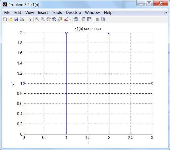
通过第1小题得到的公式计算x2序列的谱,如下:
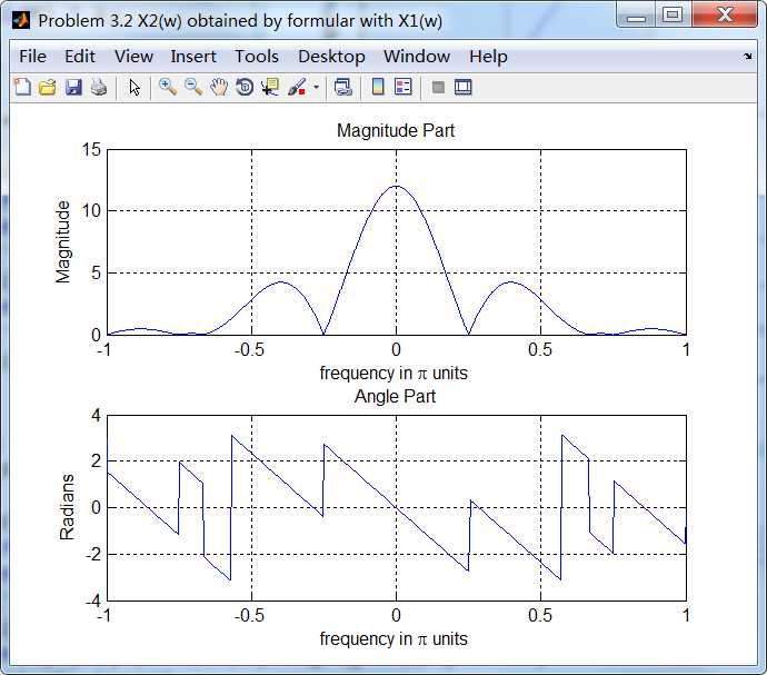
可看出,第1小题公式计算的结果,和直接将序列通过DTFT定义得到结果是相同的。