用到了三角窗脉冲序列,各小题的DTFT就不写公式了,直接画图(这里只贴长度M=10的情况)。
1、 代码:
%% ------------------------------------------------------------------------
%%            Output Info about this m-file
fprintf(‘\n***********************************************************\n‘);
fprintf(‘        <DSP using MATLAB> Problem 3.10 \n\n‘);

banner();
%% ------------------------------------------------------------------------

% --------------------------------------------------------------
%                Triangular Window sequence, and its DTFT
% --------------------------------------------------------------
M = 10;
%M = 15;
%M = 25;
%M = 100;

n1_start = 0; n1_end = M;
n1 = [n1_start : n1_end - 1];

x1 = (1 - abs(M-1-2*n1)/(M-1)) .* ones(1, length(n1));

figure(‘NumberTitle‘, ‘off‘, ‘Name‘, sprintf(‘Problem 3.10 x1(n) Triangular, M = %d‘,M));
set(gcf,‘Color‘,‘white‘);
stem(n1, x1);
xlabel(‘n‘); ylabel(‘x1‘);
title(sprintf(‘x1(n)=Tm(n) sequence, M = %d‘, M)); grid on;

MM = 500;
k = [-MM:MM];        % [-pi, pi]
%k = [0:M];        % [0, pi]
w = (pi/MM) * k;

[X1] = dtft(x1, n1, w);

magX1 = abs(X1); angX1 = angle(X1); realX1 = real(X1); imagX1 = imag(X1);


figure(‘NumberTitle‘, ‘off‘, ‘Name‘, sprintf(‘Problem 3.10 DTFT of Tm(n), M = %d‘, M));
set(gcf,‘Color‘,‘white‘);
subplot(2,1,1); plot(w/pi, magX1); grid on;
title(‘Magnitude Part‘);
xlabel(‘frequency in \pi units‘); ylabel(‘Magnitude‘);
subplot(2,1,2); plot(w/pi, angX1); grid on;
title(‘Angle Part‘);
xlabel(‘frequency in \pi units‘); ylabel(‘Radians‘);

figure(‘NumberTitle‘, ‘off‘, ‘Name‘, sprintf(‘Problem 3.10 Real and Imag of X1(w), M = %d‘, M));
set(gcf,‘Color‘,‘white‘);
subplot(‘2,1,1‘); plot(w/pi, realX1); grid on;
title(‘Real Part of X1(w)‘);
xlabel(‘frequency in \pi units‘); ylabel(‘Real‘);
subplot(‘2,1,2‘); plot(w/pi, imagX1); grid on;
title(‘Imaginary Part of X1(w)‘);
xlabel(‘frequency in \pi units‘); ylabel(‘Imaginary‘);


[X1_f, w_f] = sigfold(X1, w);
magX1f = abs(X1_f); angX1f = angle(X1_f); realX1f = real(X1_f); imagX1f = imag(X1_f);

figure(‘NumberTitle‘, ‘off‘, ‘Name‘, sprintf(‘Problem 3.10 X1(-w), M = %d‘, M));
set(gcf,‘Color‘,‘white‘);
subplot(2,1,1); plot(w_f/pi, magX1f); grid on;
title(‘Magnitude Part‘);
xlabel(‘frequency in \pi units‘); ylabel(‘Magnitude‘);
subplot(2,1,2); plot(w_f/pi, angX1f); grid on;
title(‘Angle Part‘);
xlabel(‘frequency in \pi units‘); ylabel(‘Radians‘);

figure(‘NumberTitle‘, ‘off‘, ‘Name‘, sprintf(‘Problem 3.10 Real and Imag of X1(-w), M = %d‘, M));
set(gcf,‘Color‘,‘white‘);
subplot(‘2,1,1‘); plot(w_f/pi, realX1f); grid on;
title(‘Real Part of X1(-w)‘);
xlabel(‘frequency in \pi units‘); ylabel(‘Real‘);
subplot(‘2,1,2‘); plot(w_f/pi, imagX1f); grid on;
title(‘Imaginary Part of X1(-w)‘);
xlabel(‘frequency in \pi units‘); ylabel(‘Imaginary‘);


%% ----------------------------------------------------------------
%%                 x2(n)=Tm(-n), and its DTFT
%% ----------------------------------------------------------------
[x2, n2] = sigfold(x1, n1);


figure(‘NumberTitle‘, ‘off‘, ‘Name‘, sprintf(‘Problem 3.10 x2(n), M = %d‘, M));
set(gcf,‘Color‘,‘white‘);
stem(n2, x2);
xlabel(‘n2‘); ylabel(‘x2‘);
title(sprintf(‘x2(n)=Tm(-n) sequence, M = %d‘, M)); grid on;

MM = 500;
k = [-MM:MM];        % [-pi, pi]
%k = [0:M];        % [0, pi]
w = (pi/MM) * k;

[X2] = dtft(x2, n2, w);

magX2 = abs(X2); angX2 = angle(X2); realX2 = real(X2); imagX2 = imag(X2);


figure(‘NumberTitle‘, ‘off‘, ‘Name‘, sprintf(‘Problem 3.10 DTFT of x2(n), M = %d‘, M));
set(gcf,‘Color‘,‘white‘);
subplot(2,1,1); plot(w/pi, magX2); grid on;
title(‘Magnitude Part‘);
xlabel(‘frequency in \pi units‘); ylabel(‘Magnitude‘);
subplot(2,1,2); plot(w/pi, angX2); grid on;
title(‘Angle Part‘);
xlabel(‘frequency in \pi units‘); ylabel(‘Radians‘);

figure(‘NumberTitle‘, ‘off‘, ‘Name‘, sprintf(‘Problem 3.10 Real and Imag of X2(w), M = %d‘, M));
set(gcf,‘Color‘,‘white‘);
subplot(2,1,1); plot(w/pi, realX2); grid on;
title(‘Real Part of X2(w)‘);
xlabel(‘frequency in \pi units‘); ylabel(‘Real‘);
subplot(2,1,2); plot(w/pi, imagX2); grid on;
title(‘Imaginary Part of X2(w)‘);
xlabel(‘frequency in \pi units‘); ylabel(‘Imaginary‘);
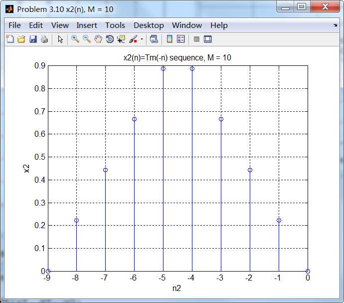
序列并进行反转得到所需题中的序列:
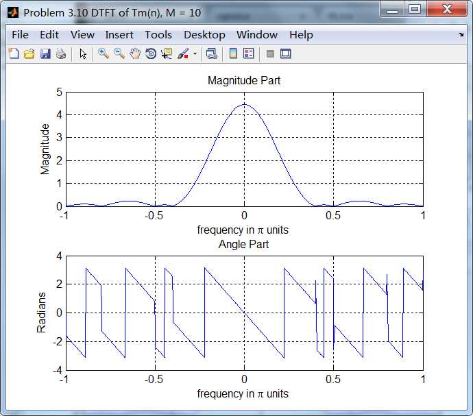
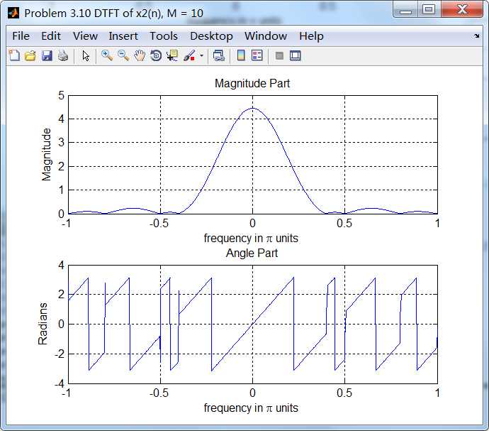
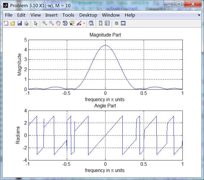
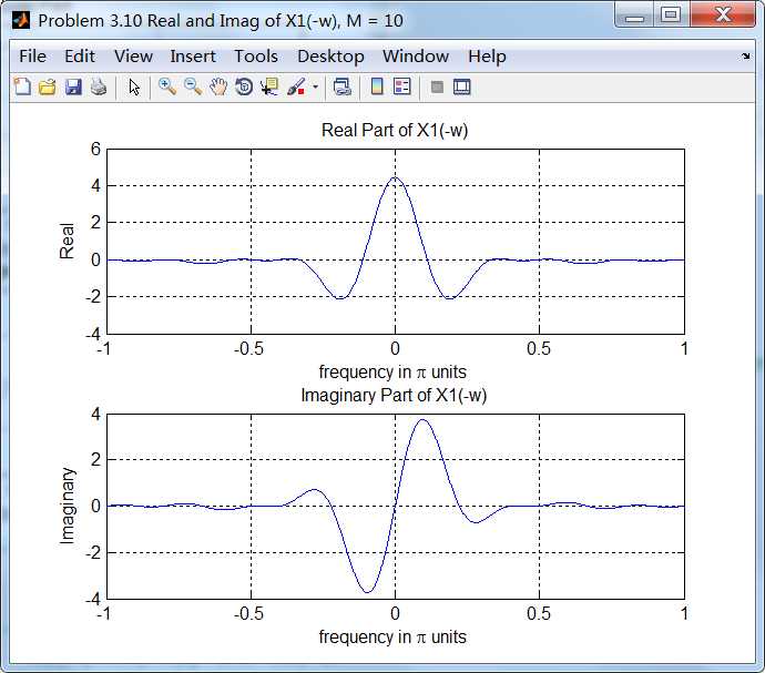
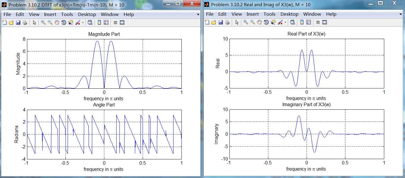
各自DTFT的幅度谱和相位谱(幅度谱相同,相位谱反相位):
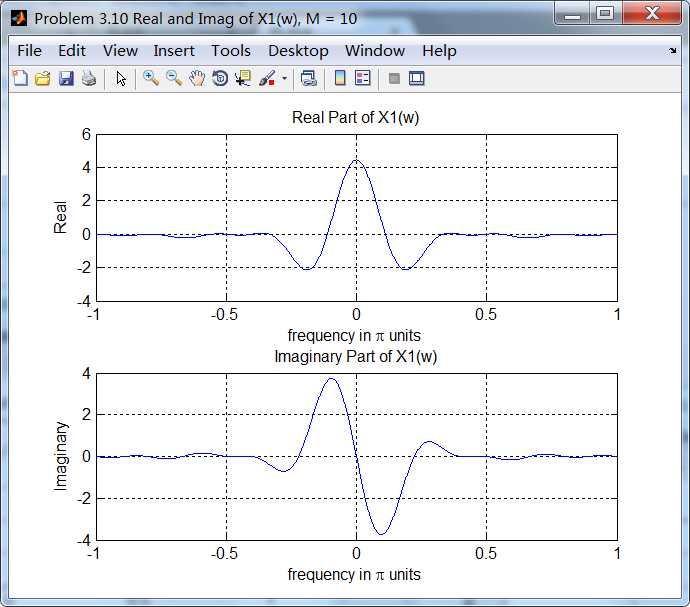
DTFT的实部和虚部:
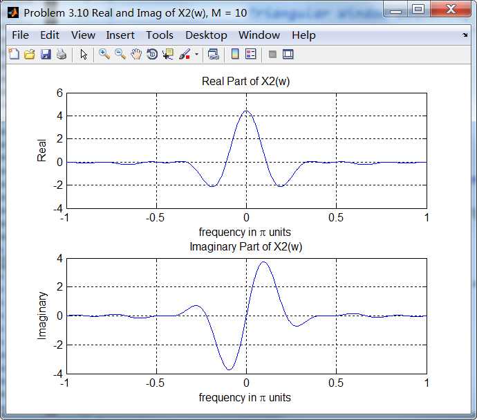
谱进行折叠;
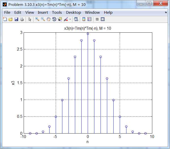
2、从第2小题到第5,序列都是由两个子序列运算而得到,以下命名都是按照第1个子序列x1(n),第2个子序列x2(n),
运算得到题目中目的序列x3(n)。
代码:
%% ------------------------------------------------------------------------
%%            Output Info about this m-file
fprintf(‘\n***********************************************************\n‘);
fprintf(‘        <DSP using MATLAB> Problem 3.10 \n\n‘);

banner();
%% ------------------------------------------------------------------------

% ------------------------------------------------------------------
%                Triangular Window sequence, and its DTFT
% ------------------------------------------------------------------
M = 10;
%M = 15;
%M = 25;
%M = 100;

n1_start = 0; n1_end = M;
n1 = [n1_start : n1_end - 1];

x1 = (1 - abs(M-1-2*n1)/(M-1)) .* ones(1, length(n1));

figure(‘NumberTitle‘, ‘off‘, ‘Name‘, sprintf(‘Problem 3.10.2 x1(n) Triangular, M = %d‘,M));
set(gcf,‘Color‘,‘white‘);
stem(n1, x1);
xlabel(‘n‘); ylabel(‘x1‘);
title(sprintf(‘x1(n)=Tm(n) sequence, M = %d‘, M)); grid on;

MM = 500;
k = [-MM:MM];        % [-pi, pi]
%k = [0:M];        % [0, pi]
w = (pi/MM) * k;

[X1] = dtft(x1, n1, w);

magX1 = abs(X1); angX1 = angle(X1); realX1 = real(X1); imagX1 = imag(X1);


figure(‘NumberTitle‘, ‘off‘, ‘Name‘, sprintf(‘Problem 3.10.2 DTFT of Tm(n), M = %d‘, M));
set(gcf,‘Color‘,‘white‘);
subplot(2,1,1); plot(w/pi, magX1); grid on;
title(‘Magnitude Part‘);
xlabel(‘frequency in \pi units‘); ylabel(‘Magnitude‘);
subplot(2,1,2); plot(w/pi, angX1); grid on;
title(‘Angle Part‘);
xlabel(‘frequency in \pi units‘); ylabel(‘Radians‘);

figure(‘NumberTitle‘, ‘off‘, ‘Name‘, sprintf(‘Problem 3.10.2 Real and Imag of X1(w), M = %d‘, M));
set(gcf,‘Color‘,‘white‘);
subplot(‘2,1,1‘); plot(w/pi, realX1); grid on;
title(‘Real Part of X1(w)‘);
xlabel(‘frequency in \pi units‘); ylabel(‘Real‘);
subplot(‘2,1,2‘); plot(w/pi, imagX1); grid on;
title(‘Imaginary Part of X1(w)‘);
xlabel(‘frequency in \pi units‘); ylabel(‘Imaginary‘);


%% -----------------------------------------------------------
%%              Tm(n-10)  and its DTFT
%% -----------------------------------------------------------
[x2, n2] = sigshift(x1, n1, 10);

figure(‘NumberTitle‘, ‘off‘, ‘Name‘, sprintf(‘Problem 3.10.2 x2(n)=Tm(n-10), M = %d‘,M));
set(gcf,‘Color‘,‘white‘);
stem(n2, x2);
xlabel(‘n‘); ylabel(‘x2‘);
title(sprintf(‘x2(n)=Tm(n-10), M = %d‘, M)); grid on;


MM = 500;
k = [-MM:MM];        % [-pi, pi]
%k = [0:M];        % [0, pi]
w = (pi/MM) * k;

[X2] = dtft(x2, n2, w);

magX2 = abs(X2); angX2 = angle(X2); realX2 = real(X2); imagX2 = imag(X2);


figure(‘NumberTitle‘, ‘off‘, ‘Name‘, sprintf(‘Problem 3.10.2 DTFT of Tm(n-10), M = %d‘, M));
set(gcf,‘Color‘,‘white‘);
subplot(2,1,1); plot(w/pi, magX2); grid on;
title(‘Magnitude Part‘);
xlabel(‘frequency in \pi units‘); ylabel(‘Magnitude‘);
subplot(2,1,2); plot(w/pi, angX2); grid on;
title(‘Angle Part‘);
xlabel(‘frequency in \pi units‘); ylabel(‘Radians‘);

figure(‘NumberTitle‘, ‘off‘, ‘Name‘, sprintf(‘Problem 3.10.2 Real and Imag of X2(w), M = %d‘, M));
set(gcf,‘Color‘,‘white‘);
subplot(2,1,1); plot(w/pi, realX2); grid on;
title(‘Real Part of X2(w)‘);
xlabel(‘frequency in \pi units‘); ylabel(‘Real‘);
subplot(2,1,2); plot(w/pi, imagX2); grid on;
title(‘Imaginary Part of X2(w)‘);
xlabel(‘frequency in \pi units‘); ylabel(‘Imaginary‘);


%% -------------------------------------------------------------
%%            Tm(n)-Tm(n-10) and its DTFT
%% -------------------------------------------------------------
[x3, n3] = sigadd(x1, n1, -x2, n2);

figure(‘NumberTitle‘, ‘off‘, ‘Name‘, sprintf(‘Problem 3.10.2 x3(n)=Tm(n)-Tm(n-10), M = %d‘,M));
set(gcf,‘Color‘,‘white‘);
stem(n3, x3);
xlabel(‘n‘); ylabel(‘x3‘);
title(sprintf(‘x3(n)=Tm(n)-Tm(n-10), M = %d‘, M)); grid on;


MM = 500;
k = [-MM:MM];        % [-pi, pi]
%k = [0:M];        % [0, pi]
w = (pi/MM) * k;

[X3] = dtft(x3, n3, w);

magX3 = abs(X3); angX3 = angle(X3); realX3 = real(X3); imagX3 = imag(X3);


figure(‘NumberTitle‘, ‘off‘, ‘Name‘, sprintf(‘Problem 3.10.2 DTFT of x3(n)=Tm(n)-Tm(n-10), M = %d‘, M));
set(gcf,‘Color‘,‘white‘);
subplot(2,1,1); plot(w/pi, magX3); grid on;
title(‘Magnitude Part‘);
xlabel(‘frequency in \pi units‘); ylabel(‘Magnitude‘);
subplot(2,1,2); plot(w/pi, angX3); grid on;
title(‘Angle Part‘);
xlabel(‘frequency in \pi units‘); ylabel(‘Radians‘);

figure(‘NumberTitle‘, ‘off‘, ‘Name‘, sprintf(‘Problem 3.10.2 Real and Imag of X3(w), M = %d‘, M));
set(gcf,‘Color‘,‘white‘);
subplot(‘2,1,1‘); plot(w/pi, realX3); grid on;
title(‘Real Part of X3(w)‘);
xlabel(‘frequency in \pi units‘); ylabel(‘Real‘);
subplot(‘2,1,2‘); plot(w/pi, imagX3); grid on;
title(‘Imaginary Part of X3(w)‘);
xlabel(‘frequency in \pi units‘); ylabel(‘Imaginary‘);


%% ------------------------------------------------------
%%           Properties of DTFT
%% ------------------------------------------------------
X3_check = X1 - X1 .* exp(-j * w * 10);

magX3C = abs(X3_check); angX3C = angle(X3_check); realX3C = real(X3_check); imagX3C = imag(X3_check);

figure(‘NumberTitle‘, ‘off‘, ‘Name‘, sprintf(‘Problem 3.10.2 DTFT[Tm(n)]-DTFT[Tm(n-10)], M = %d‘, M));
set(gcf,‘Color‘,‘white‘);
subplot(2,1,1); plot(w/pi, magX3C); grid on;
title(‘Magnitude Part‘);
xlabel(‘frequency in \pi units‘); ylabel(‘Magnitude‘);
subplot(2,1,2); plot(w/pi, angX3C); grid on;
title(‘Angle Part‘);
xlabel(‘frequency in \pi units‘); ylabel(‘Radians‘);

figure(‘NumberTitle‘, ‘off‘, ‘Name‘, sprintf(‘Problem 3.10.2 Real and Imag of X3C(w), M = %d‘, M));
set(gcf,‘Color‘,‘white‘);
subplot(‘2,1,1‘); plot(w/pi, realX3C); grid on;
title(‘Real Part of X3_check(w)‘);
xlabel(‘frequency in \pi units‘); ylabel(‘Real‘);
subplot(‘2,1,2‘); plot(w/pi, imagX3C); grid on;
title(‘Imaginary Part of X3_check(w)‘);
xlabel(‘frequency in \pi units‘); ylabel(‘Imaginary‘);
运行结果:
3、代码
%% ------------------------------------------------------------------------
%%            Output Info about this m-file
fprintf(‘\n***********************************************************\n‘);
fprintf(‘        <DSP using MATLAB> Problem 3.10 \n\n‘);

banner();
%% ------------------------------------------------------------------------

% ------------------------------------------------------------------
%                Triangular Window sequence, and its DTFT
% ------------------------------------------------------------------
M = 10;
%M = 15;
%M = 25;
%M = 100;

n1_start = 0; n1_end = M;
n1 = [n1_start : n1_end - 1];

x1 = (1 - abs(M-1-2*n1)/(M-1)) .* ones(1, length(n1));

figure(‘NumberTitle‘, ‘off‘, ‘Name‘, sprintf(‘Problem 3.10.3 x1(n) Triangular, M = %d‘,M));
set(gcf,‘Color‘,‘white‘);
stem(n1, x1);
xlabel(‘n‘); ylabel(‘x1‘);
title(sprintf(‘x1(n)=Tm(n) sequence, M = %d‘, M)); grid on;

MM = 500;
k = [-MM:MM];        % [-pi, pi]
%k = [0:M];        % [0, pi]
w = (pi/MM) * k;

[X1] = dtft(x1, n1, w);

magX1 = abs(X1); angX1 = angle(X1); realX1 = real(X1); imagX1 = imag(X1);


figure(‘NumberTitle‘, ‘off‘, ‘Name‘, sprintf(‘Problem 3.10.3 DTFT of Tm(n), M = %d‘, M));
set(gcf,‘Color‘,‘white‘);
subplot(2,1,1); plot(w/pi, magX1); grid on;
title(‘Magnitude Part‘);
xlabel(‘frequency in \pi units‘); ylabel(‘Magnitude‘);
subplot(2,1,2); plot(w/pi, angX1); grid on;
title(‘Angle Part‘);
xlabel(‘frequency in \pi units‘); ylabel(‘Radians‘);

figure(‘NumberTitle‘, ‘off‘, ‘Name‘, sprintf(‘Problem 3.10.3 Real and Imag of X1(w), M = %d‘, M));
set(gcf,‘Color‘,‘white‘);
subplot(‘2,1,1‘); plot(w/pi, realX1); grid on;
title(‘Real Part of X1(w)‘);
xlabel(‘frequency in \pi units‘); ylabel(‘Real‘);
subplot(‘2,1,2‘); plot(w/pi, imagX1); grid on;
title(‘Imaginary Part of X1(w)‘);
xlabel(‘frequency in \pi units‘); ylabel(‘Imaginary‘);


%% ---------------------------------------------------------------
%%                  Tm(-n)  and its DTFT
%% ---------------------------------------------------------------
[x2, n2] = sigfold(x1, n1);

figure(‘NumberTitle‘, ‘off‘, ‘Name‘, sprintf(‘Problem 3.10.3 x2(n)=Tm(-n), M = %d‘,M));
set(gcf,‘Color‘,‘white‘);
stem(n2, x2);
xlabel(‘n‘); ylabel(‘x2‘);
title(sprintf(‘x2(n)=Tm(-n), M = %d‘, M)); grid on;


MM = 500;
k = [-MM:MM];        % [-pi, pi]
%k = [0:M];        % [0, pi]
w = (pi/MM) * k;

[X2] = dtft(x2, n2, w);

magX2 = abs(X2); angX2 = angle(X2); realX2 = real(X2); imagX2 = imag(X2);


figure(‘NumberTitle‘, ‘off‘, ‘Name‘, sprintf(‘Problem 3.10.3 DTFT of Tm(-n), M = %d‘, M));
set(gcf,‘Color‘,‘white‘);
subplot(2,1,1); plot(w/pi, magX2); grid on;
title(‘Magnitude Part‘);
xlabel(‘frequency in \pi units‘); ylabel(‘Magnitude‘);
subplot(2,1,2); plot(w/pi, angX2); grid on;
title(‘Angle Part‘);
xlabel(‘frequency in \pi units‘); ylabel(‘Radians‘);

figure(‘NumberTitle‘, ‘off‘, ‘Name‘, sprintf(‘Problem 3.10.3 Real and Imag of X2(w)=X1(-w), M = %d‘, M));
set(gcf,‘Color‘,‘white‘);
subplot(2,1,1); plot(w/pi, realX2); grid on;
title(‘Real Part of X2(w)‘);
xlabel(‘frequency in \pi units‘); ylabel(‘Real‘);
subplot(2,1,2); plot(w/pi, imagX2); grid on;
title(‘Imaginary Part of X2(w)‘);
xlabel(‘frequency in \pi units‘); ylabel(‘Imaginary‘);


%% -----------------------------------------------------------------
%%                 Tm(n)*Tm(-n) and its DTFT
%% -----------------------------------------------------------------
[x3, n3] = conv_m(x1, n1, x2, n2);

figure(‘NumberTitle‘, ‘off‘, ‘Name‘, sprintf(‘Problem 3.10.3 x3(n)=Tm(n)*Tm(-n), M = %d‘,M));
set(gcf,‘Color‘,‘white‘);
stem(n3, x3);
xlabel(‘n‘); ylabel(‘x3‘);
title(sprintf(‘x3(n)=Tm(n)*Tm(-n), M = %d‘, M)); grid on;


MM = 500;
k = [-MM:MM];        % [-pi, pi]
%k = [0:M];        % [0, pi]
w = (pi/MM) * k;

[X3] = dtft(x3, n3, w);

magX3 = abs(X3); angX3 = angle(X3); realX3 = real(X3); imagX3 = imag(X3);


figure(‘NumberTitle‘, ‘off‘, ‘Name‘, sprintf(‘Problem 3.10.3 DTFT of x3(n)=Tm(n)*Tm(-n), M = %d‘, M));
set(gcf,‘Color‘,‘white‘);
subplot(2,1,1); plot(w/pi, magX3); grid on;
title(‘Magnitude Part‘);
xlabel(‘frequency in \pi units‘); ylabel(‘Magnitude‘);
subplot(2,1,2); plot(w/pi, angX3); grid on;
title(‘Angle Part‘);
xlabel(‘frequency in \pi units‘); ylabel(‘Radians‘);

figure(‘NumberTitle‘, ‘off‘, ‘Name‘, sprintf(‘Problem 3.10.3 Real and Imag of X3(w), M = %d‘, M));
set(gcf,‘Color‘,‘white‘);
subplot(‘2,1,1‘); plot(w/pi, realX3); grid on;
title(‘Real Part of X3(w)‘);
xlabel(‘frequency in \pi units‘); ylabel(‘Real‘);
subplot(‘2,1,2‘); plot(w/pi, imagX3); grid on;
title(‘Imaginary Part of X3(w)‘);
xlabel(‘frequency in \pi units‘); ylabel(‘Imaginary‘);


%% ------------------------------------------------------
%%           Properties of DTFT
%% ------------------------------------------------------
%[X3_check, m] = sigmult(X1, w/pi*500, X2, w/pi*500);
X3_check = X1 .* X2;

magX3C = abs(X3_check); angX3C = angle(X3_check); realX3C = real(X3_check); imagX3C = imag(X3_check);

figure(‘NumberTitle‘, ‘off‘, ‘Name‘, sprintf(‘Problem 3.10.3 DTFT[Tm(n)]XDTFT[Tm(-n)], M = %d‘, M));
set(gcf,‘Color‘,‘white‘);
subplot(2,1,1); plot(w/pi, magX3C); grid on;
title(‘Magnitude Part‘);
xlabel(‘frequency in \pi units‘); ylabel(‘Magnitude‘);
subplot(2,1,2); plot(w/pi, angX3C); grid on;
title(‘Angle Part‘);
xlabel(‘frequency in \pi units‘); ylabel(‘Radians‘);

figure(‘NumberTitle‘, ‘off‘, ‘Name‘, sprintf(‘Problem 3.10.3 Real and Imag of X3C(w), M = %d‘, M));
set(gcf,‘Color‘,‘white‘);
subplot(‘2,1,1‘); plot(w/pi, realX3C); grid on;
title(‘Real Part of X3 check(w)‘);
xlabel(‘frequency in \pi units‘); ylabel(‘Real‘);
subplot(‘2,1,2‘); plot(w/pi, imagX3C); grid on;
title(‘Imaginary Part of X3 check(w)‘);
xlabel(‘frequency in \pi units‘); ylabel(‘Imaginary‘);
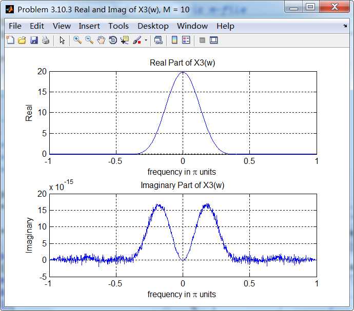
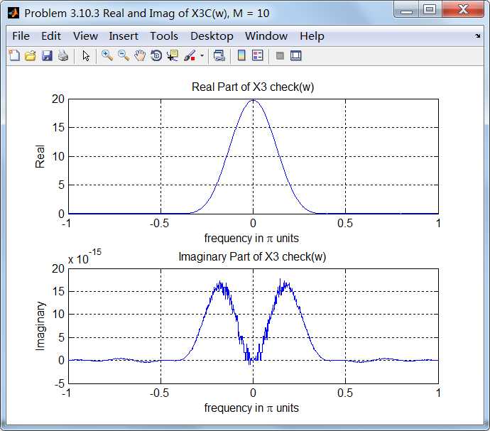
运行结果:
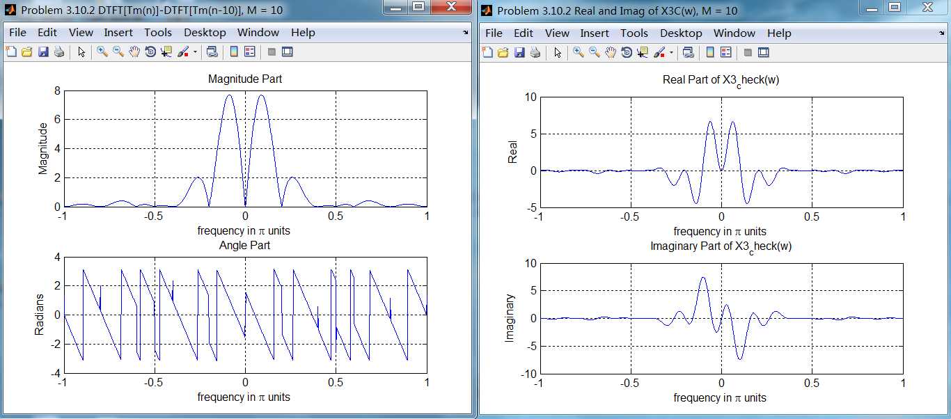
卷积后求DTFT,其实部和虚部:
先求各自DTFT再相乘,虚部稍有不同;
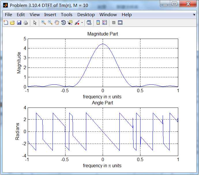
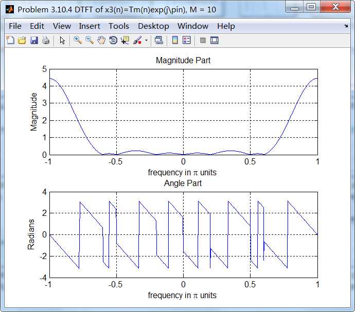
4、代码:
%% ------------------------------------------------------------------------
%%            Output Info about this m-file
fprintf(‘\n***********************************************************\n‘);
fprintf(‘        <DSP using MATLAB> Problem 3.10 \n\n‘);

banner();
%% ------------------------------------------------------------------------

% ------------------------------------------------------------------
%                Triangular Window sequence, and its DTFT
% ------------------------------------------------------------------
M = 10;
%M = 15;
%M = 25;
%M = 100;

n1_start = 0; n1_end = M;
n1 = [n1_start : n1_end - 1];

x1 = (1 - abs(M-1-2*n1)/(M-1)) .* ones(1, length(n1));

figure(‘NumberTitle‘, ‘off‘, ‘Name‘, sprintf(‘Problem 3.10.4 x1(n) Triangular, M = %d‘,M));
set(gcf,‘Color‘,‘white‘);
stem(n1, x1);
xlabel(‘n‘); ylabel(‘x1‘);
title(sprintf(‘x1(n)=Tm(n) sequence, M = %d‘, M)); grid on;

MM = 500;
k = [-MM:MM];        % [-pi, pi]
%k = [0:M];        % [0, pi]
w = (pi/MM) * k;

[X1] = dtft(x1, n1, w);

magX1 = abs(X1); angX1 = angle(X1); realX1 = real(X1); imagX1 = imag(X1);


figure(‘NumberTitle‘, ‘off‘, ‘Name‘, sprintf(‘Problem 3.10.4 DTFT of Tm(n), M = %d‘, M));
set(gcf,‘Color‘,‘white‘);
subplot(2,1,1); plot(w/pi, magX1); grid on;
title(‘Magnitude Part‘);
xlabel(‘frequency in \pi units‘); ylabel(‘Magnitude‘);
subplot(2,1,2); plot(w/pi, angX1); grid on;
title(‘Angle Part‘);
xlabel(‘frequency in \pi units‘); ylabel(‘Radians‘);

figure(‘NumberTitle‘, ‘off‘, ‘Name‘, sprintf(‘Problem 3.10.4 Real and Imag of X1(w), M = %d‘, M));
set(gcf,‘Color‘,‘white‘);
subplot(‘2,1,1‘); plot(w/pi, realX1); grid on;
title(‘Real Part of X1(w)‘);
xlabel(‘frequency in \pi units‘); ylabel(‘Real‘);
subplot(‘2,1,2‘); plot(w/pi, imagX1); grid on;
title(‘Imaginary Part of X1(w)‘);
xlabel(‘frequency in \pi units‘); ylabel(‘Imaginary‘);


%% ---------------------------------------------------------------
%%                  exp(jπn)  and its DTFT
%% ---------------------------------------------------------------
n2 = n1;
x2 = exp(j*pi*n2);

figure(‘NumberTitle‘, ‘off‘, ‘Name‘, sprintf(‘Problem 3.10.4 x2(n)=exp(j%\pin), M = %d‘,M));
set(gcf,‘Color‘,‘white‘);
subplot(2,1,1); stem(n2, real(x2));
xlabel(‘n‘); ylabel(‘x2‘);
title(sprintf(‘Real part x2(n)=exp(j\\pin), M = %d‘, M)); grid on;
subplot(2,1,2); stem(n2, imag(x2));
xlabel(‘n‘); ylabel(‘x2‘);
title(sprintf(‘Imaginary part x2(n)=exp(j\\pin), M = %d‘, M)); grid on;


MM = 500;
k = [-MM:MM];        % [-pi, pi]
%k = [0:M];        % [0, pi]
w = (pi/MM) * k;

[X2] = dtft(x2, n2, w);

magX2 = abs(X2); angX2 = angle(X2); realX2 = real(X2); imagX2 = imag(X2);


figure(‘NumberTitle‘, ‘off‘, ‘Name‘, sprintf(‘Problem 3.10.4 DTFT of exp(j\\pin), M = %d‘, M));
set(gcf,‘Color‘,‘white‘);
subplot(2,1,1); plot(w/pi, magX2); grid on;
title(‘Magnitude Part‘);
xlabel(‘frequency in \pi units‘); ylabel(‘Magnitude‘);
subplot(2,1,2); plot(w/pi, angX2); grid on;
title(‘Angle Part‘);
xlabel(‘frequency in \pi units‘); ylabel(‘Radians‘);

figure(‘NumberTitle‘, ‘off‘, ‘Name‘, sprintf(‘Problem 3.10.4 Real and Imag of X2(w), M = %d‘, M));
set(gcf,‘Color‘,‘white‘);
subplot(2,1,1); plot(w/pi, realX2); grid on;
title(‘Real Part of X2(w)‘);
xlabel(‘frequency in \pi units‘); ylabel(‘Real‘);
subplot(2,1,2); plot(w/pi, imagX2); grid on;
title(‘Imaginary Part of X2(w)‘);
xlabel(‘frequency in \pi units‘); ylabel(‘Imaginary‘);


%% -----------------------------------------------------------------
%%                 Tm(n)*exp(jπn) and its DTFT
%% -----------------------------------------------------------------
[x3, n3] = sigmult(x1, n1, x2, n2);

figure(‘NumberTitle‘, ‘off‘, ‘Name‘, sprintf(‘Problem 3.10.4 x3(n)=Tm(n)exp(j\\pin), M = %d‘,M));
set(gcf,‘Color‘,‘white‘);
subplot(2,1,1); stem(n3, real(x3));
xlabel(‘n‘); ylabel(‘x3‘);
title(sprintf(‘Real part x3(n)=Tm(n)exp(j\\pin), M = %d‘, M)); grid on;
subplot(2,1,2); stem(n3, imag(x3));
xlabel(‘n‘); ylabel(‘x3‘);
title(sprintf(‘Imaginary part x3(n)=Tm(n)exp(j\\pin), M = %d‘, M)); grid on;


MM = 500;
k = [-MM:MM];        % [-pi, pi]
%k = [0:M];        % [0, pi]
w = (pi/MM) * k;

[X3] = dtft(x3, n3, w);

magX3 = abs(X3); angX3 = angle(X3); realX3 = real(X3); imagX3 = imag(X3);


figure(‘NumberTitle‘, ‘off‘, ‘Name‘, sprintf(‘Problem 3.10.4 DTFT of x3(n)=Tm(n)exp(j\\pin), M = %d‘, M));
set(gcf,‘Color‘,‘white‘);
subplot(2,1,1); plot(w/pi, magX3); grid on;
title(‘Magnitude Part‘);
xlabel(‘frequency in \pi units‘); ylabel(‘Magnitude‘);
subplot(2,1,2); plot(w/pi, angX3); grid on;
title(‘Angle Part‘);
xlabel(‘frequency in \pi units‘); ylabel(‘Radians‘);

figure(‘NumberTitle‘, ‘off‘, ‘Name‘, sprintf(‘Problem 3.10.4 Real and Imag of X3(w), M = %d‘, M));
set(gcf,‘Color‘,‘white‘);
subplot(‘2,1,1‘); plot(w/pi, realX3); grid on;
title(‘Real Part of X3(w)‘);
xlabel(‘frequency in \pi units‘); ylabel(‘Real‘);
subplot(‘2,1,2‘); plot(w/pi, imagX3); grid on;
title(‘Imaginary Part of X3(w)‘);
xlabel(‘frequency in \pi units‘); ylabel(‘Imaginary‘);


%% ------------------------------------------------------
%%           Properties of DTFT
%% ------------------------------------------------------

[X3_check, n3_check] = sigshift(X1, w/pi*500, pi/pi);

magX3C = abs(X3_check); angX3C = angle(X3_check); realX3C = real(X3_check); imagX3C = imag(X3_check);

figure(‘NumberTitle‘, ‘off‘, ‘Name‘, sprintf(‘Problem 3.10.4 X3C=X1(w-\\pi), M = %d‘, M));
set(gcf,‘Color‘,‘white‘);
%subplot(2,1,1); plot(w/pi, magX3C);
subplot(2,1,1); plot(n3_check/500*pi, magX3C);
title(‘Magnitude Part‘);
xlabel(‘frequency in \pi units‘); ylabel(‘Magnitude‘); grid on;
axis([-1,1,-1,6]);
%subplot(2,1,2); plot(w/pi, angX3C);
subplot(2,1,2); plot(n3_check/500*pi, angX3C);
title(‘Angle Part‘);
xlabel(‘frequency in \pi units‘); ylabel(‘Radians‘); grid on;
axis([-1,1,-8,8]);

figure(‘NumberTitle‘, ‘off‘, ‘Name‘, sprintf(‘Problem 3.10.4 Real and Imag of X3C(w), M = %d‘, M));
set(gcf,‘Color‘,‘white‘);
%subplot(‘2,1,1‘); plot(w/pi, realX3C); grid on;
subplot(‘2,1,1‘); plot(n3_check/500*pi, realX3C); grid on;
title(‘Real Part of X3 check(w)‘);
xlabel(‘frequency in \pi units‘); ylabel(‘Real‘);
axis([-1,1,-4,6]);
%subplot(‘2,1,2‘); plot(w/pi, imagX3C); grid on;
subplot(‘2,1,2‘); plot(n3_check/500*pi, imagX3C); grid on;
title(‘Imaginary Part of X3 check(w)‘);
xlabel(‘frequency in \pi units‘); ylabel(‘Imaginary‘);
运行结果:
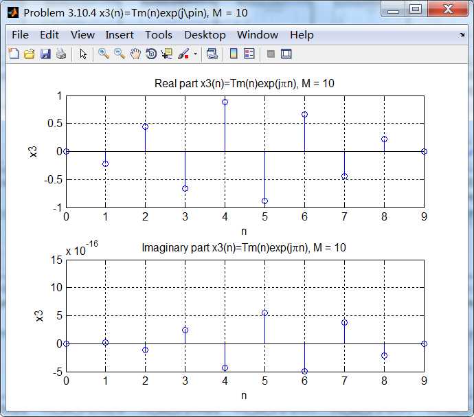
三角窗序列乘以复指数序列,相当于谱频移了(这里是π):
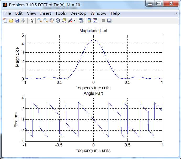
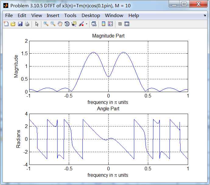
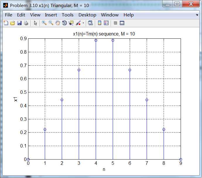
5、代码:
%% ------------------------------------------------------------------------
%%            Output Info about this m-file
fprintf(‘\n***********************************************************\n‘);
fprintf(‘        <DSP using MATLAB> Problem 3.10 \n\n‘);

banner();
%% ------------------------------------------------------------------------

% ------------------------------------------------------------------
%                Triangular Window sequence, and its DTFT
% ------------------------------------------------------------------
M = 10;
%M = 15;
%M = 25;
%M = 100;

n1_start = 0; n1_end = M;
n1 = [n1_start : n1_end - 1];

x1 = (1 - abs(M-1-2*n1)/(M-1)) .* ones(1, length(n1));

figure(‘NumberTitle‘, ‘off‘, ‘Name‘, sprintf(‘Problem 3.10.5 x1(n) Triangular, M = %d‘,M));
set(gcf,‘Color‘,‘white‘);
stem(n1, x1);
xlabel(‘n‘); ylabel(‘x1‘);
title(sprintf(‘x1(n)=Tm(n) sequence, M = %d‘, M)); grid on;

MM = 500;
k = [-MM:MM];        % [-pi, pi]
%k = [0:M];        % [0, pi]
w = (pi/MM) * k;

[X1] = dtft(x1, n1, w);

magX1 = abs(X1); angX1 = angle(X1); realX1 = real(X1); imagX1 = imag(X1);


figure(‘NumberTitle‘, ‘off‘, ‘Name‘, sprintf(‘Problem 3.10.5 DTFT of Tm(n), M = %d‘, M));
set(gcf,‘Color‘,‘white‘);
subplot(2,1,1); plot(w/pi, magX1); grid on;
title(‘Magnitude Part‘);
xlabel(‘frequency in \pi units‘); ylabel(‘Magnitude‘);
subplot(2,1,2); plot(w/pi, angX1); grid on;
title(‘Angle Part‘);
xlabel(‘frequency in \pi units‘); ylabel(‘Radians‘);

figure(‘NumberTitle‘, ‘off‘, ‘Name‘, sprintf(‘Problem 3.10.5 Real and Imag of X1(w), M = %d‘, M));
set(gcf,‘Color‘,‘white‘);
subplot(‘2,1,1‘); plot(w/pi, realX1); grid on;
title(‘Real Part of X1(w)‘);
xlabel(‘frequency in \pi units‘); ylabel(‘Real‘);
subplot(‘2,1,2‘); plot(w/pi, imagX1); grid on;
title(‘Imaginary Part of X1(w)‘);
xlabel(‘frequency in \pi units‘); ylabel(‘Imaginary‘);


%% ---------------------------------------------------------------
%%                  cos(0.1πn)  and its DTFT
%% ---------------------------------------------------------------
n2 = n1;
x2 = cos(0.1*pi*n2);

figure(‘NumberTitle‘, ‘off‘, ‘Name‘, sprintf(‘Problem 3.10.5 x2(n)=cos(0.1pin), M = %d‘,M));
set(gcf,‘Color‘,‘white‘);
stem(n2, x2);
xlabel(‘n‘); ylabel(‘x2‘);
title(sprintf(‘x2(n)=cos(0.1pin), M = %d‘, M)); grid on;


MM = 500;
k = [-MM:MM];        % [-pi, pi]
%k = [0:M];        % [0, pi]
w = (pi/MM) * k;

[X2] = dtft(x2, n2, w);

magX2 = abs(X2); angX2 = angle(X2); realX2 = real(X2); imagX2 = imag(X2);


figure(‘NumberTitle‘, ‘off‘, ‘Name‘, sprintf(‘Problem 3.10.5 DTFT of cos(0.1pin), M = %d‘, M));
set(gcf,‘Color‘,‘white‘);
subplot(2,1,1); plot(w/pi, magX2); grid on;
title(‘Magnitude Part‘);
xlabel(‘frequency in \pi units‘); ylabel(‘Magnitude‘);
subplot(2,1,2); plot(w/pi, angX2); grid on;
title(‘Angle Part‘);
xlabel(‘frequency in \pi units‘); ylabel(‘Radians‘);

figure(‘NumberTitle‘, ‘off‘, ‘Name‘, sprintf(‘Problem 3.10.5 Real and Imag of X2(w), M = %d‘, M));
set(gcf,‘Color‘,‘white‘);
subplot(2,1,1); plot(w/pi, realX2); grid on;
title(‘Real Part of X2(w)‘);
xlabel(‘frequency in \pi units‘); ylabel(‘Real‘);
subplot(2,1,2); plot(w/pi, imagX2); grid on;
title(‘Imaginary Part of X2(w)‘);
xlabel(‘frequency in \pi units‘); ylabel(‘Imaginary‘);


%% -----------------------------------------------------------------
%%                 Tm(n)*cos(0.1πn) and its DTFT
%% -----------------------------------------------------------------
[x3, n3] = sigmult(x1, n1, x2, n2);
%x3 = x1 .* x2;

figure(‘NumberTitle‘, ‘off‘, ‘Name‘, sprintf(‘Problem 3.10.5 x3(n)=Tm(n)cos(0.1pin), M = %d‘,M));
set(gcf,‘Color‘,‘white‘);
subplot(2,1,1); stem(n3, real(x3));
xlabel(‘n‘); ylabel(‘x3‘);
title(sprintf(‘Real part x3(n)=Tm(n)cos(0.1pin), M = %d‘, M)); grid on;
subplot(2,1,2); stem(n3, imag(x3));
xlabel(‘n‘); ylabel(‘x3‘);
title(sprintf(‘Imaginary part x3(n)=Tm(n)cos(0.1pin), M = %d‘, M)); grid on;


MM = 500;
k = [-MM:MM];        % [-pi, pi]
%k = [0:M];        % [0, pi]
w = (pi/MM) * k;

[X3] = dtft(x3, n3, w);

magX3 = abs(X3); angX3 = angle(X3); realX3 = real(X3); imagX3 = imag(X3);


figure(‘NumberTitle‘, ‘off‘, ‘Name‘, sprintf(‘Problem 3.10.5 DTFT of x3(n)=Tm(n)cos(0.1pin), M = %d‘, M));
set(gcf,‘Color‘,‘white‘);
subplot(2,1,1); plot(w/pi, magX3); grid on;
title(‘Magnitude Part‘);
xlabel(‘frequency in \pi units‘); ylabel(‘Magnitude‘);
subplot(2,1,2); plot(w/pi, angX3); grid on;
title(‘Angle Part‘);
xlabel(‘frequency in \pi units‘); ylabel(‘Radians‘);

figure(‘NumberTitle‘, ‘off‘, ‘Name‘, sprintf(‘Problem 3.10.5 Real and Imag of X3(w), M = %d‘, M));
set(gcf,‘Color‘,‘white‘);
subplot(‘2,1,1‘); plot(w/pi, realX3); grid on;
title(‘Real Part of X3(w)‘);
xlabel(‘frequency in \pi units‘); ylabel(‘Real‘);
subplot(‘2,1,2‘); plot(w/pi, imagX3); grid on;
title(‘Imaginary Part of X3(w)‘);
xlabel(‘frequency in \pi units‘); ylabel(‘Imaginary‘);


%% ------------------------------------------------------
%%           Properties of DTFT
%% ------------------------------------------------------

[X3_check, n3_check] = sigshift(X1, w/pi*500, pi/pi);

magX3C = abs(X3_check); angX3C = angle(X3_check); realX3C = real(X3_check); imagX3C = imag(X3_check);

figure(‘NumberTitle‘, ‘off‘, ‘Name‘, sprintf(‘Problem 3.10.4 X3C=X1(w-\\pi), M = %d‘, M));
set(gcf,‘Color‘,‘white‘);
%subplot(2,1,1); plot(w/pi, magX3C);
subplot(2,1,1); plot(n3_check/500*pi, magX3C);
title(‘Magnitude Part‘);
xlabel(‘frequency in \pi units‘); ylabel(‘Magnitude‘); grid on;
axis([-1,1,-1,6]);
%subplot(2,1,2); plot(w/pi, angX3C);
subplot(2,1,2); plot(n3_check/500*pi, angX3C);
title(‘Angle Part‘);
xlabel(‘frequency in \pi units‘); ylabel(‘Radians‘); grid on;
axis([-1,1,-8,8]);

figure(‘NumberTitle‘, ‘off‘, ‘Name‘, sprintf(‘Problem 3.10.4 Real and Imag of X3C(w), M = %d‘, M));
set(gcf,‘Color‘,‘white‘);
%subplot(‘2,1,1‘); plot(w/pi, realX3C); grid on;
subplot(‘2,1,1‘); plot(n3_check/500*pi, realX3C); grid on;
title(‘Real Part of X3 check(w)‘);
xlabel(‘frequency in \pi units‘); ylabel(‘Real‘);
axis([-1,1,-4,6]);
%subplot(‘2,1,2‘); plot(w/pi, imagX3C); grid on;
subplot(‘2,1,2‘); plot(n3_check/500*pi, imagX3C); grid on;
title(‘Imaginary Part of X3 check(w)‘);
xlabel(‘frequency in \pi units‘); ylabel(‘Imaginary‘);
运行结果:
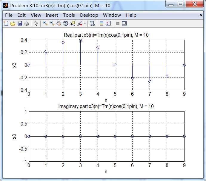
序列与余弦函数cos(ω0n)相乘,相当于原序列的频谱频移了ω0=0.1π个单位: