绝大部分机翻,少部分手动矫正,仅供参考。本人水平有限,如有误翻,概不负责。。。
Position Based Dynamics
Abstract
The most popular approaches for the simulation of dynamic systems in computer graphics are force based. Internal and external forces are accumulated from which accelerations are computed based on Newton’s second law of motion. A time integration method is then used to update the velocities and finally the positions of the object. A few simulation methods (most rigid body simulators) use impulse based dynamics and directly manipulate velocities. In this paper we present an approach which omit the velocity layer as well and immediately works on the positions. The main advantage of a position based approach is its controllability. Overshooting problems of explicit integration schemes in force based systems can be avoided. In addition, collision constraints can be handled easily and penetrations can be resolved completely by projecting points to valid locations. We have used the approach to build a real time cloth simulator which is part of a physics software library for games. This application demonstrates the strengths and benefits of the method.
计算机图形学中最常用的动态系统仿真方法是基于力的。内部和外部的力是根据牛顿第二运动定律计算得到的加速度。然后使用时间积分方法来更新速度,最后更新对象的位置。一些仿真方法(多数刚体模拟器)使用基于脉冲的动力学,直接操纵速度。本文提出了一种将速度层忽略的方法,并立即应用于位置。基于位置的方法的主要优点是它的可控性。可以避免在基于force的系统中出现显式积分方案的问题。此外,可以很容易地处理碰撞约束,通过投射点到有效位置可以完全解决穿透性问题。我们用这种方法构建了一个实时的布匹模拟器,它是游戏物理软件库的一部分。这个应用程序展示了该方法的强项和便利处。
1. Introduction
Research in the field of physically based animation in computer graphics is concerned with finding new methods for the simulation of physical phenomena such as the dynamics of rigid bodies, deformable objects or fluid flow. In contrast to computational sciences where the main focus is on accuracy, the main issues here are stability, robustness and speed while the results should remain visually plausible. Therefore, existing methods from computational sciences can not be adopted one to one. In fact, the main justification for doing research on physically based simulation in computer graphics is to come up with specialized methods, tailored to the particular needs in the field. The method we present falls into this category.
在计算机图形学的物理基动画领域的研究发现了物理现象的模拟方法,如刚体动力学、可变形物体或流体流动。与主要关注精度的计算科学相反,这里的主要问题是稳定性、健壮性和速度,而结果应该在视觉上看起来可信。因此,现有的计算科学方法不能一对一地采用。事实上,在计算机图形学的物理基础上进行研究的主要理由是提出专门的方法,专门针对该领域的特定需求。我们提出的方法属于这一类。
The traditional approach to simulating dynamic objects has been to work with forces. At the beginning of each time step, internal and external forces are accumulated. Examples of internal forces are elastic forces in deformable objects or viscosity and pressure forces in fluids. Gravity and collision forces are examples of external forces. Newton’s second law of motion relates forces to accelerations via the mass. So using the density or lumped masses of vertices, the forces are transformed into accelerations. Any time integration scheme can then be used to first compute the velocities from the accelerations and then the positions from the velocities. Some approaches use impulses instead of forces to control the animation. Because impulses directly change velocities, one level of integration can be skipped.
模拟动态对象的传统方法基于力进行的。在每一步开始的时候,内部和外部的力就会累积起来。内力的例子是形变物体的弹性力或流体的粘性和压力。重力和碰撞力是外力的例子。牛顿运动的第二定律是通过质量来促进加速度。因此,利用密度或集中质量的顶点,将力转化为加速度。任何时间积分方案都可以用来首先计算加速度的速度,然后是速度的位置。有些方法用脉冲而不是力来控制动画。因为脉冲直接改变速度,所以可以跳过一阶积分。
In computer graphics and especially in computer games it is often desirable to have direct control over positions of objects or vertices of a mesh. The user might want to attach a vertex to a kinematic object or make sure the vertex always stays outside a colliding object. The method we propose here works directly on positions which makes such manipulations easy. In addition, with the position based approach it is possible to control the integration directly thereby avoiding overshooting and energy gain problems in connection with explicit integration. So the main features and advantages of position based dynamics are
- Position based simulation gives control over explicit integration and removes the typical instability problems.
- Positions of vertices and parts of objects can directly be manipulated during the simulation.
- The formulation we propose allows the handling of general constraints in the position based setting.
- The explicit position based solver is easy to understand and implement.
在计算机图形学,特别是在计算机游戏中,通常需要直接控制网格的对象或顶点的位置。用户可能想要将一个顶点附加到一个运动物体上,或者确定顶点总是在碰撞物体外面。我们在这里提出的方法直接作用于位置,而使这种操作更容易。此外,基于位置的方法,可以直接控制积分,从而避免了显式积分的过度问题和能量增益问题。因此,基于位置的动力学的主要特征和优势是
- 基于位置的仿真给出了显式积分的控制,消除了典型的不稳定性问题。
- 在模拟过程中,顶点和对象部分的位置可以直接被操纵。
- 我们建议的公式允许在基于位置的设置中处理一般的约束。
- 基于明确位置的solver很容易理解和实现。
2. Related Work
3. Position Based Simulation
In this section we will formulate the general position based approach. With cloth simulation, we will give a particular application of the method in the subsequent and in the results section. We consider a three dimensional world. However, the approach works equally well in two dimensions.
在本节中,我们将阐述基于总体立场的方法。在布模拟的情况下,我们将在后续的和结果部分中给出具体的方法应用。我们考虑一个三维世界。然而,这种方法在二维世界同样有效。
3.1. Algorithm Overview
We represent a dynamic object by a set of \(N\) vertices and \(M\) constraints. A vertex \(i\in [1,\cdots ,N]\) has a mass \(m_i\), a position \(\mathbf x_i\) and a velocity \(\mathbf v_i\).A constraint \(j\in [1,\ldots ,M]\) consists of
我们通过一组\(N\)个顶点和\(M\)个约束来表示一个动态对象。对于一个顶点\(i\in [1,\cdots,N]\)有质量\(m_i\),位置\(\mathbf x_i\)和速度\(\mathbf v_i\)。每一个约束\(j\in [1,\ldots ,M]\) 由以下组成
- a cardinality \(n_j\),
基数(和该约束相关的顶点的个数)\(n_j\), - a function \(C_j:\mathbb R^{3n_j} \to \mathbb R\),
约束函数\(C_j:\mathbb R^{3n_j} \to \mathbb R\), - a set of indices \(\{i_1,\ldots i_{n_j}\}, i_k \in [1,\ldots N]\),
相关顶点索引集合\(\{i_1,\ldots i_{n_j}\}, i_k \in [1,\ldots N]\), - a stiffness parameter \(k_j \in [0 \ldots 1]\) and
刚度系数\(k_j \in [0 \ldots 1]\) - a type of either equality or inequality.
以及约束类型,equality 或者 inequality。
Constraint \(j\) with type equality is satisfied if \(C_j(\mathbf x_{i_1},\ldots ,x_{i_{n_j}}) = 0\). If its type is inequality then it is satisfied if \(C_j(\mathbf x_{i_1},\ldots ,x_{i_{n_j}}) \ge 0\). The stiffness parameter \(k_j\) defines the strength of the constraint in a range from zero to one.
如果约束\(j\)的类型为equality,则约束函数应满足\(C_j(\mathbf x_{i_1},\ldots,x_{i_{n_j}})=0\)。如果类型是inequality,那么约束函数应满足\(C_j(\mathbf x_{i_1},\ldots,x_{i_{n_j}})\ge 0\)。刚度参数\(k_j\)定义了约束强度,范围从0到1。
Based on this data and a time step \(\Delta t\), the dynamic object is simulated as follows:
基于此数据和时间步长\(\Delta t\),动态对象模拟过程如下:
(01) forall vertices \(i\)
(02) initialize \(\mathbf x_i = \mathbf x^0_i,\mathbf v_i = \mathbf v^0_i,w_i = 1/m_i\)
(03) endfor
(04) loop
(05) forall vertices \(i\) do \(\mathbf v_i \gets \mathbf v_i +\Delta t w_i \mathbf f_{ext}(\mathbf x_i)\)
(06) dampVelocities(\(\mathbf v_1,\ldots ,\mathbf v_N\))
(07) forall vertices \(i\) do \(\mathbf p_i \gets \mathbf x_i + \Delta t \mathbf v_i\)
(08) forall vertices \(i\) do generateCollisionConstraints(\(\mathbf x_i \to \mathbf p_i\))
(09) loop solverIterations times
(10) projectConstraints(\(C_1,\ldots ,C_{M+M_{coll}}, \mathbf p_1,\ldots ,\mathbf p_N\))
(11) endloop
(12) forall vertices \(i\)
(13) \(\mathbf v_i \gets (\mathbf p_i - \mathbf x_i)/ \Delta t\)
(14) \(\mathbf x_i \gets \mathbf p_i\)
(15) endfor
(16) velocityUpdate(\(\mathbf v_1,\ldots,\mathbf v_N\))
(17) endloop
Lines (1)-(3) just initialize the state variables. The core idea of position based dynamics is shown in lines (7), (9)-(11) and (13)-(14). In line (7), estimates \(\mathbf p_i\) for new locations of the vertices are computed using an explicit Euler integration step. The iterative solver (9)-(11) manipulates these position estimates such that they satisfy the constraints. It does this by repeatedly project each constraint in a GaussSeidel type fashion (see Section 3.2). In steps (13) and (14), the positions of the vertices are moved to the optimized estimates and the velocities are updated accordingly. This is in exact correspondence with a Verlet integration step and a modification of the current position [Jak01], because the Verlet method stores the velocity implicitly as the difference between the current and the last position. However, working with velocities allows for a more intuitive way of manipulating them.
行(1)-(3)只是初始化状态变量。PBD的主要思想位于(7)、(9)-(11)和(13)-(14)。在第(7)行中,使用显示欧拉积分的方法来预估位置\(\mathbf p_i\)。可迭代的solver(9)-(11)操作这些预估位置,使它们满足约束条件。它通过反复地以GaussSeidel类型的方式来完成每个约束(参见第3.2节)。在步骤(13)和(14)中,顶点的位置被移动到优化的估计值,并相应地更新速度。这与Verlet积分步骤和当前位置[Jak01]的修改是完全一致的,因为Verlet方法将速度隐式地存储为当前和最后一个位置之间的差。然而,使用速度允许更直观的操作方法。
The velocities are manipulated in line (5), (6) and (16). Line (5) allows to hook up external forces to the system if some of the forces cannot be converted to positional constraints. We only use it to add gravity to the system in which case the line becomes \(\mathbf v_i \gets \mathbf v_i + \Delta t\mathbf g\), where \(\mathbf g\) is the gravitational acceleration. In line (6), the velocities can be damped if this is necessary. In Section 3.5 we show how to add global damping without influencing the rigid body modes of the object. Finally, in line (16), the velocities of colliding vertices are modified according to friction and restitution coefficients.
在行(5)、(6)和(16)中对速度进行了操作。如果某些力不能转化为位置约束,可以在行(5)中将外力与系统连接起来。如果外力只有重力,那么行(5)可以改为\(\mathbf v_i \gets \mathbf v_i + \Delta t\mathbf g\), 其中\(\mathbf g\)是重力加速度。在第(6)行中,可以为速度添加阻尼响应。在第3.5节中,我们展示了如何在不影响物体的刚体模式的情况下增加全局阻尼。最后,在行(16)中,根据摩擦系数和补偿系数对碰撞顶点的速度进行了修正。
The given constraints \(C_1,\ldots ,C_M\) are fixed throughout the simulation. In addition to these constraints, line (8) generates the \(M_{coll}\) collision constraints which change from time step to time step. The projection step in line (10) considers both, the fixed and the collision constraints.
给定的约束\(C_1,\ldots,C_M\)在整个模拟过程中是固定数目的。除了这些约束条件外,在第行(8)每帧都会动态的生成\(M_{coll}\)个碰撞约束。行(10)的Projection操作则考虑了全部的约束,固定数目的约束和碰撞产生的约束。
The scheme is unconditionally stable. This is because the integration steps (13) and (14) do not extrapolate blindly into the future as traditional explicit schemes do but move the vertices to a physically valid configuration \(\mathbf p_i\) computed by the constraint solver. The only possible source for instabilities is the solver itself which uses the Newton-Raphson method to solve for valid positions (see Section 3.3). However, its stability does not depend on the time step size but on the shape of the constraint functions.
该方案是无条件稳定的。这是因为积分步骤(13)和(14)不像传统的显式积分方案那样盲目地推断结果,而是将每个顶点首先移动到物理上有效的位置\(\mathbf p_i\),该位置是由约束solver计算。唯一造成不稳定性的来源,只可能是solver在求解有效位置的过程中,采用的Newton-Raphson方法(参见第3.3节)。不管怎样,它的稳定性是并不依赖于时间步长的,而是取决于约束函数的构造。
The integration does not fall clearly into the category of implicit or explicit schemes. If only one solver iteration is performed per time step, it looks more like an explicit scheme. By increasing the number of iterations, however, a constrained system can be made arbitrarily stiff and the algorithm behaves more like an implicit scheme. Increasing the number of iterations shifts the bottleneck from collision detection to the solver.
这种积分方法不属于隐式或显式模式的范畴。如果每帧只执行一次solver迭代,那么它看起来更像是一个显式的方案。然而,通过增加迭代次数,可以使约束系统变得任意强壮,而该算法的行为更像是一个隐式方案。增加迭代次数将瓶颈从碰撞检测转移到solver。
3.2. The Solver
The input to the solver are the \(M+M_{coll}\) constraints and the estimates \(\mathbf p_1,\ldots,\mathbf p_N\) for the new locations of the points. The solver tries to modify the estimates such that they satisfy all the constraints. The resulting system of equations is non-linear. Even a simple distance constraint \(C(\mathbf p_1,\mathbf p_2) = |\mathbf p_1 - \mathbf p_2| - d\) yields a non-linear equation. In addition, the constraints of type inequality yield inequalities. To solve such a general set of equations and inequalities, we use a Gauss-Seidel-type iteration. The original Gauss-Seidel algorithm (GS) can only handle linear system. The part we borrow from GS is the idea of solving each constraint independently one after the other. However, in contrast to GS,solving a constraint is a non linear operation. We repeatedly iterate through all the constraints and project the particles to valid locations with respect to the given constraint alone. In contrast to a Jacobi-type iteration, modifications to point locations immediately get visible to the process. This speeds up convergence significantly because pressure waves can propagate through the material in a single solver step, an effect which is dependent on the order in which constraints are solved. In over-constrained situations, the process can lead to oscillations if the order is not kept constant.
solver的输入是\(M+M_{coll}\)个约束,和作为顶点新位移的一组预估位置\(\mathbf p_1,\ldots,\mathbf p_N\)。solver会尝试修改这些预估位置,使其满足所有约束条件。由此产生的方程组是非线性的。即使是一个简单的距离约束\(C(\mathbf p_1,\mathbf p_2) = |\mathbf p_1 - \mathbf p_2| - d\)也会生成一个非线性方程。此外,类型为inequality的约束也会产生不等式。为了解决这样一组方程和不等式,我们使用了Gauss-Seidel类型的迭代法。原始的Gauss-Seidel算法(GS)只能解决线性系统问题。我们从GS中借用的思想,是相继地独立解决每个约束(GS算法是将前面求解的结果应用到未求解的等式中,应该是这个意思吧)。然而,与GS相比,求解约束是一个非线性的操作。我们反复遍历所有的约束,并将粒子投影到有效的位置,仅考虑给定的约束条件。与雅可比迭代法相比,对点位置的修改可以立即对过程可见。这大大加快了收敛速度,因为压力波可以在一个单独的求解过程中通过材料传播,这种效应依赖于约束求解的顺序。在过度约束的情况下,如果顺序不保持不变,则过程可能导致振荡。
3.3. Constraint Projection
Projecting a set of points according to a constraint means moving the points such that they satisfy the constraint. The most important issue in connection with moving points directly inside a simulation loop is the conservation of linear and angular momentum. Let \(\Delta \mathbf p_i\) be the displacement of vertex \(i\) by the projection. Linear momentum is conserved if
根据约束投影一组点,也就是说移动这些点来满足约束。在模拟循环中与移动点相关的最重要的问题,是如何保持线性动量守恒和角动量守恒。令\(\Delta \mathbf p_i\)为顶点\(i\)的Projection位移(应该就是Projection之后的位移差)。线性动量守恒的条件为
\[\sum_i m_i \Delta \mathbf p_i = \mathbf 0 \tag{1}\]
which amounts to conserving the center of mass. Angular momentum is conserved if
也就是基于质心守恒。角动量守恒的条件为
\[\sum_i \mathbf r_i \times m_i \Delta \mathbf p_i = \mathbf 0 \tag{2}\]
where the \(\mathbf r_i\) are the distances of the \(\mathbf p_i\) to an arbitrary common rotation center. If a projection violates one of these constraints, it introduces so called ghost forces which act like external forces dragging and rotation the object. However, only internal constraints need to conserve the momenta. Collision or attachment constraints are allowed to have global effects on the object.
其中\(\mathbf r_i\)是\(\mathbf p_i\)到任意旋转中心(如何任意?)的距离。如果一个Projection违反了其中的一个约束条件,它就会引入所谓的ghost force,表现得像外力拖动和旋转物体一样。然而,只有内部约束需要保持动量守恒。碰撞或附加约束允许对对象产生全局影响。
The method we propose for constraint projection conserves both momenta for internal constraints. Again, the point based approach is more direct in that we can directly use the constraint function while force based methods derive forces via an energy term (see [BW98, THMG04]). Let us look at a constraint with cardinality \(n\) on the points \(\mathbf p_1, \ldots ,\mathbf p_n\) with constraint function \(C\) and stiffness \(k\). We let \(\mathbf p\) be the concatenation \([\mathbf p^T_1, \ldots , \mathbf p^T_n]^T\). For internal constraints, \(C\) is independent of rigid body modes, i.e. translation and rotation. This means that rotating or translating the points does not change the value of the constraint function. Therefore, the gradient \(\nabla_{\mathbf p}C\) is perpendicular to rigid body modes because it is the direction of maximal change. If the correction \(\Delta \mathbf p\) is chosen to be along \(\nabla_{\mathbf p}C\) both momenta are automatically conserved if all masses are equal (we handle different masses later). Given \(\mathbf p\) we want to find a correction \({\Delta \mathbf p}\) such that \(C(\mathbf p + \Delta \mathbf p) = 0\). This equation can be approximated by
我们提出的约束投影的方法既可以满足内部约束条件,又可以满足动量守恒的要求。同样,基于点的方法更直接,因为我们可以直接使用约束函数,而基于力的方法则通过能量部分驱使力的作用(见[BW98,THMG04])。让我们在基数为\(n\)的点集\(\mathbf p_1, \ldots ,\mathbf p_n\)中,单独分析一个刚度系数为\(k\)的约束\(C\)。我们令\(\mathbf p\)表示为\([\mathbf p^T_1, \ldots , \mathbf p^T_n]^T\)。对于内部约束,\(C\)和刚体的平移和旋转无关。这意味着旋转或平移点集不会改变约束函数的值。因此,梯度\(\nabla_{\mathbf p}C\)垂直于刚体模式,因为它是最大变化的方向。在所有点质量相等的情况下(稍后我们处理不同的质量),如果校正量\(\Delta \mathbf p\)是沿着\(\nabla_{\mathbf p}C\)的方向,那么所有的动量都会自动保持守恒。给定\(\mathbf p\)我们想求出一个校正量\({\Delta \mathbf p}\),满足\(C(\mathbf p + \Delta \mathbf p) = 0\)。这个方程可以近似为
\[C(\mathbf p + \Delta \mathbf p) \approx C(\mathbf p) + \nabla_{\mathbf p}C(\mathbf p) \cdot \Delta \mathbf p = 0 \tag{3}\]
Restricting \(\Delta \mathbf p\) to be in the direction of \(\nabla_{\mathbf p}C\) means choosing a scalar \(\lambda\) such that
限制\(\Delta \mathbf p\)在\(\nabla_{\mathbf p}C\)的方向上,也就是说存在标量\(\lambda\)可以令
\[ \Delta \mathbf p = \lambda \nabla_{\mathbf p}C(\mathbf p) \tag{4}\]
Substituting Eq.(4) into Eq.(3), solving for \(\lambda\) and substituting it back into Eq.(4) yields the final formula for \(\Delta \mathbf p\)
将公式(4)带入公式(3)求出\(\lambda\),并将其代入回公式(4)中,可以得到最终的公式求\(\Delta \mathbf p\)
\[\Delta \mathbf p = - \frac{C(\mathbf p)}{|\nabla_{\mathbf p}C(\mathbf p)|^2} \nabla_{\mathbf p}C(\mathbf p) \tag{5}\]
which is a regular Newton-Raphson step for the iterative solution of the non-linear equation given by a single constraint. For the correction of an individual point \(\mathbf p_i\) we have
公式(5)是一个正规的牛顿迭代步骤,迭代求解给定单个约束的非线性方程。对于单独的点\(\mathbf p_i\)的矫正值如下
\[\Delta \mathbf p_i = -s\nabla_{\mathbf p_i}C(\mathbf p_1,\ldots,\mathbf p_n), \tag{6}\]
where the scaling factor
缩放系数为
\[s = \frac{C(\mathbf p_1,\ldots,\mathbf p_n)}{\sum_j| \nabla_{\mathbf p_j}C(\mathbf p_1,\ldots,\mathbf p_n)|^2} \tag{7}\]
is the same for all points. If the points have individual masses, we weight the corrections \(\Delta \mathbf p_i\) by the inverse masses \(w_i=1/m_i\). In this case a point with infinite mass, i.e. wi = 0, does not move for example as expected. Now Eq. (4) is replaced by
对于所有点都是一样的。如果这些点有不同的质量,我们通过质量的倒数\(w_i=1/m_i\)作为校正量\(\Delta \mathbf p_i\)的权重值。如果一个点的质量无限大即\(w_i=0\),那么就不对其进行移动。现在公式(4)可以被替换为
\(\Delta \mathbf p_i = \lambda w_i \nabla_{\mathbf p_i} C(\mathbf p)\) yielding
\[s = \frac{C(\mathbf p_1,\ldots,\mathbf p_n)}{\sum_j w_j| \nabla_{\mathbf p_j}C(\mathbf p_1,\ldots,\mathbf p_n)|^2} \tag{8}\]
for the scaling factor and for the final correction
最终方程为
\[\Delta \mathbf p_i = -sw_i\nabla_{\mathbf p_i}C(\mathbf p_1,\ldots,\mathbf p_n). \tag{9}\]
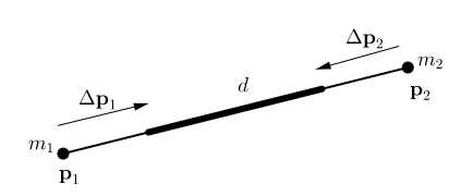
To give an example, let us consider the distance constraint function \(C(\mathbf p_1, \mathbf p_2)=|\mathbf p_1 - \mathbf p_2|-d\). The derivative with respect to the points are \(\nabla_{\mathbf p_1}C(\mathbf p_1, \mathbf p_2)=\mathbf n\) and \(\nabla_{\mathbf p_2}C(\mathbf p_1, \mathbf p_2)=\mathbf -\mathbf n\) with \(\mathbf n=\frac{\mathbf p_1-\mathbf p_2}{|\mathbf p_1-\mathbf p_2|}\). The scaling factor \(s\) is, thus, \(s = \frac{|\mathbf p_1 - \mathbf p_2|-d}{w_1+w_2}\) and the final corrections
举个栗子,考虑一个距离约束函数为 \(C(\mathbf p_1, \mathbf p_2)=|\mathbf p_1 - \mathbf p_2|-d\)。约束函数对点的微分分别为:\(\nabla_{\mathbf p_1}C(\mathbf p_1, \mathbf p_2)=\mathbf n\) 和 \(\nabla_{\mathbf p_2}C(\mathbf p_1, \mathbf p_2)=-\mathbf n\),其中 \(\mathbf n=\frac{\mathbf p_1-\mathbf p_2}{|\mathbf p_1-\mathbf p_2|}\)。缩放系数\(s\)的公式为\(s = \frac{|\mathbf p_1 - \mathbf p_2|-d}{w_1+w_2}\),最后矫正变量公式如下:
\[\Delta \mathbf p_1 = -\frac{w_1}{w_1+w_2}(|\mathbf p_1 - \mathbf p_2|-d)\frac{\mathbf p_1-\mathbf p_2}{|\mathbf p_1-\mathbf p_2|} \tag{10}\]
\[\Delta \mathbf p_2 = +\frac{w_1}{w_1+w_2}(|\mathbf p_1 - \mathbf p_2|-d)\frac{\mathbf p_1-\mathbf p_2}{|\mathbf p_1-\mathbf p_2|} \tag{11}\]
which are the formulas proposed in [Jak01] for the projection of distance constraints (see Figure 2). They pop up as a
special case of the general constraint projection method.
这是[Jak01]中提出的距离约束投影的公式(见 Figure 2),它们作为一般约束投影方法的特例出现。
We have not considered the type and the stiffness \(k\) of the constraint so far. Type handling is straight forward. If the type is equality we always perform a projection. If the type is inequality, the projection is only performed if \(C(\mathbf p_1,\ldots,\mathbf p_n)<0\). There are several ways of incorporating the stiffness parameter. The simplest variant is to multiply the corrections \(\Delta \mathbf p\) by \(k\in[0 \ldots 1]\). However, for multiple iteration loops of the solver, the effect of \(k\) is non-linear. The remaining error for a single distance constraint after \(n_s\) solver iterations is \(\Delta \mathbf p(1-k)^{n_s}\). To get a linear relationship we multiply the corrections not by \(k\) directly but by \(k'=1-(1-k)^{1/n_s}\). With this transformation the error becomes \(\Delta \mathbf p(1-k')^{n_s}=\Delta \mathbf p(1-k)\) and, thus, becomes linearly dependent on \(k\) and independent of \(n_s\) as desired. However, the resulting material stiffness is still dependent on the time step of the simulation. Real time environments typically use fixed time steps in which case this dependency is not problematic.
到目前为止,我们还没有考虑到约束的类型和刚度\(k\)。对于约束类型的处理方法很直接。如果类型是equality我们就直接去执行Projection。如果类型是inequality,则Projection只在\(C(\mathbf p_1,\ldots,\mathbf p_n)<0\)时执行。有几种方法可以结合刚度参数。最简单的方法是用\(\Delta \mathbf p\)去和\(k\in[0 \ldots 1]\)相乘。然而,对于求解器的多重迭代循环,\(k\)的影响是非线性的。在\(n_s\)求解迭代后,单距离约束的剩余误差是\(\Delta \mathbf p(1-k)^{n_s}\)。为了得到一种线性关系,我们将修正不是直接乘以\(k\),而是乘以\(k'=1-(1-k)^{1/n_s}\)。在这个变换中,误差变成了\(\Delta \mathbf p(1-k')^{n_s}=\Delta \mathbf p(1-k)\),从而线性依赖于\(k\),并与\(n_s\)无关。然而,得到的材料刚度仍然取决于模拟的时间步长。实时环境通常使用固定的时间步骤,在这种情况下,这种依赖是没有问题的。
3.4. Collision Detection and Response
One advantage of the position based approach is how simply collision response can be realized. In line (8) of the simulation algorithm the \(M_{coll}\) collision constraints are generated. While the first \(M\) constraints given by the object representation are fixed throughout the simulation, the additional \(M_{coll}\) constraints are generated from scratch at each time step. The number of collision constraints \(M_{coll}\) varies and depends on the number of colliding vertices. Both, continuous and static collisions can be handled. For continuous collision handling, we test for each vertex \(i\) the ray \(\mathbf x_i \to \mathbf p_i\). If this ray enters an object, we compute the entry point \(\mathbf q_c\) and the surface normal \(\mathbf n_c\) at this position. An inequality constraint with constraint function \(C(\mathbf p) = (\mathbf p - \mathbf q_c) \cdot \mathbf n_c\) and stiffness \(k = 1\) is added to the list of constraints. If the ray \(\mathbf x_i \to \mathbf p_i\) lies completely inside an object, continuous collision detection has failed at some point. In this case we fall back to static collision handling. We compute the surface point \(\mathbf q_s\) which is closest to \(\mathbf p_i\) and the surface normal \(\mathbf n_s\) at this position. An inequality constraint with constraint function \(C(\mathbf p) = (\mathbf p - \mathbf q_s) \cdot \mathbf n_s\) and stiffness \(k=1\) is added to the list of constraints. Collision constraint generation is done outside of the solver loop. This makes the simulation much faster. There are certain scenarios, however, where collisions can be missed if the solver works with a fixed collision constraint set. Fortunately, according to our experience, the artifacts are negligible.
基于位置的方法的一个优点是可以简单地实现碰撞响应。在仿真算法的第8行中,生成了\(M_{coll}\)个碰撞约束。虽然在整个模拟过程中,对象表示所给出的前\(M\)个约束是固定的,但是在每次步骤中都需要从头开始生成额外的\(M_{coll}\)个约束。碰撞约束的数量\(M_{coll}\)是变化的,并且取决于碰撞顶点的个数。连续碰撞和静态碰撞都可以进行处理。对于连续的碰撞处理,我们测试每个顶点\(i\)进行射线测试,射线为\(\mathbf x_i \to \mathbf p_i\)。如果这条射线进入一个物体,我们将计算对应的入口点\(\mathbf q_c\)和表面法线\(\mathbf n_c\)。添加一个inequality的约束添加到约束的队列中,其约束函数为\(C(\mathbf p) = (\mathbf p - \mathbf q_c) \cdot \mathbf n_c\),刚度\(k=1\)。如果射线\(\mathbf x_i \to \mathbf p_i\)完全在一个对象内,连续碰撞检测则失败了。在这种情况下,我们回到静态碰撞处理。我们计算距离\(\mathbf p_i\)最近的表面点\(\mathbf q_s\),对应的表面法线为\(\mathbf n_s\)。添加一个inequality的约束添加到约束的队列中,其约束函数为\(C(\mathbf p) = (\mathbf p - \mathbf q_s) \cdot \mathbf n_s\),刚度\(k=1\)。碰撞约束在solver循环之外生成结束了。这使得模拟的速度更快。但是在某些场景中,如果solver使用固定的碰撞约束集,就可以忽略冲突。幸运的是,根据我们的经验,这些问题是可以忽略的。
Friction and restitution can be handled by manipulating the velocities of colliding vertices in step (16) of the algorithm. The velocity of each vertex for which a collision constraint has been generated is dampened perpendicular to the collision normal and reflected in the direction of the collision normal.
在算法的步骤(16)中,通过控制碰撞顶点的速度来处理摩擦和补偿。由碰撞约束产生的顶点速度与碰撞的法线垂直,并且与碰撞法线方向相反。
The collision handling discussed above is only correct for collisions with static objects because no impulse is transferred to the collision partners. Correct response for two dynamic colliding objects can be achieved by simulating both objects with our simulator, i.e. the \(N\) vertices and \(M\) constraints which are the input to our algorithm simply represent two or more independent objects. Then, if a point \(\mathbf q\) of one objects moves through a triangle \(\mathbf p_1, \mathbf p_2, \mathbf p_3\) of another object, we insert an inequality constraint with constraint function \(C(\mathbf q, \mathbf p_1, \mathbf p_2, \mathbf p_3) = \pm (\mathbf q - \mathbf p_1) \cdot [(\mathbf p_2 - \mathbf p_1) \times (\mathbf p_3 - \mathbf p_1)]\) which keeps the point \(\mathbf q\) on the correct side of the triangle. Since this constraint function is independent of rigid body modes, it will correctly conserve linear and angular momentum. Collision detection gets slightly more involved because the four vertices are represented by rays \(\mathbf x_i \to \mathbf p_i\). Therefore the collision of a moving point against a moving triangle needs to be detected (see section about cloth self collision).
上面讨论的碰撞处理仅适用于与静态物体碰撞,因为没有将任何冲力传递给该碰撞体(因为是静态对象嘛)。对于两个动态碰撞体的正确碰撞响应,可以通过我们的模拟器来模拟双方来实现,例如,作为算法的输入,\(N\)个顶点和\(M\)个约束可以代表2个或者更多的独立对象。如果其中一个对象的点\(\mathbf q\)穿过了另一个对象中的三角形\(\mathbf p_1, \mathbf p_2, \mathbf p_3\),我们插入一个inequality类型的约束,约束函数为\(C(\mathbf q, \mathbf p_1, \mathbf p_2, \mathbf p_3) = \pm (\mathbf q - \mathbf p_1) \cdot [(\mathbf p_2 - \mathbf p_1) \times (\mathbf p_3 - \mathbf p_1)]\),可以保证点\(\mathbf q\)在三角形正确的一面。既然这个约束函数是与刚体模式无关的,那么它可以正确的保持线性量和角动量。碰撞检测涉及更多,因为4个顶点可以表示射线\(\mathbf x_i \to \mathbf p_i\)。因此,需要检测移动点与移动三角形的碰撞(参见有关布料自碰撞的部分)。
3.5. Damping
In line (6) of the simulation algorithm the velocities are dampened before they are used for the prediction of the new positions. Any form of damping can be used and many methods for damping have been proposed in the literature (see [NMK05]). Here we propose a new method with some interesting properties:
在模拟算法的第(6)行中,速度在用于预测新位置之前进行的阻力计算。任何形式的阻力都可以应用,并且这些阻力的方法已经在文献[NMK05]中提出。这里我们提出了一种新的方法,具有一些有趣的特性:
(1) \(\mathbf x_{cm} = (\sum_i \mathbf x_i m_i)/(\sum_i m_i)\)
(2) \(\mathbf v_{cm} = (\sum_i \mathbf v_i m_i)/(\sum_i m_i)\)
(3) \(\mathbf L = \sum_i \mathbf r_i \times (m_i \mathbf v_i)\)
(4) \(\mathbf I = \sum_i \mathbf{\tilde r}_i \mathbf{\tilde r}^T_i m_i\)
(5) \(\omega = \mathbf I^{-1}\mathbf L\)
(6) forall vertices \(i\)
(7) \(\Delta \mathbf v_i = \mathbf v_{cm} + \omega \times \mathbf r_i - \mathbf v_i\)
(8) \(\mathbf v_i \gets \mathbf v_i + k_{\text{damping}}\Delta \mathbf v_i\)
(9) endfor
Here \(\mathbf r_i = \mathbf x_i - \mathbf x_{cm}\), \(\mathbf {\tilde r}_i\) is the 3 by 3 matrix with the property \(\mathbf {\tilde r}_i \mathbf v = \mathbf r_i \times \mathbf v\), and \(k_{\text{damping}} \in [0 \ldots 1]\) is the damping coefficient. In lines (1)-(5) we compute the global linear velocity \(\mathbf x_{cm}\) and angular velocity \(\omega\) of the system. Lines (6)-(9) then only damp the individual deviations \(\Delta v_i\) of the velocities \(\mathbf v_i\) from the global motion \(\mathbf v_{cm} + \omega \times \mathbf r_i\). Thus, in the extreme case \(k_{\text{damping}} = 1\) , only the global motion survives and the set of vertices behaves like a rigid body. For arbitrary values of \(k_{\text{damping}}\), the velocities are globally dampened but without influencing the global motion of the vertices.
这里\(\mathbf r_i = \mathbf x_i - \mathbf x_{cm}\),\(\mathbf {\tilde r}_i\)是一个3阶矩阵,隐式表达式为\(\mathbf {\tilde r}_i \mathbf v = \mathbf r_i \times \mathbf v\),\(k_{\text{damping}} \in [0 \ldots 1]\)为阻尼系数。在(1)-(5)行中,我们计算了系统的全局线性速度\(\mathbf x_{cm}\)和角速度\(\omega\)。行(6)-(9)依据全局的动量\(\mathbf v_{cm} + \omega \times \mathbf r_i\)来计算速度\(\mathbf v_i\)的阻尼差值\(\Delta v_i\)。在\(k_{\text{damping}} = 1\)的极端条件下,只有全局动量保存,并且可以使顶点表现的如同刚体一般。对于变量\(k_{\text{damping}}\),速度可以在不影响顶点全局动量的情况下,接受速度阻尼。
3.6. Attachments
With the position based approach, attaching vertices to static or kinematic objects is quite simple. The position of the vertex is simply set to the static target position or updated at every time step to coincide with the position of the kinematic object. To make sure other constraints containing this vertex do not move it, its inverse mass \(w_i\) is set to zero.
基于位置的方法,将顶点附加到静态或运动学对象非常简单(其实最常见的应该就是固定顶点与拖拽顶点之类的)。顶点的位置简单地设置为静态目标位置(固定住顶点),或者每帧更新对应的运动对象的位置(运动对象,鼠标之类的吧,或者场景中运动物体)。为了确保被附加的顶点不会被包含该点的其他约束不移动它,顶点质量的倒数\(w_i\)可设置为零。
4. Cloth Simulation
We have used the point based dynamics framework to implement a real time cloth simulator for games. In this section we will discuss cloth specific issues thereby giving concrete examples of the general concepts introduced in the previous section.
我们使用了基于点的动态框架来实现游戏的实时布料模拟器。在本节中,我们将讨论布的具体问题,从而给出上一节介绍的一般概念的具体例子。
4.1. Representation of Cloth
Our cloth simulator accepts as input arbitrary triangle meshes. The only restriction we impose on the input mesh is that it represents a manifold, i.e. each edge is shared by at most two triangles. Each node of the mesh becomes a simulated vertex. The user provides a density \(\rho\) given in mass per area [\(kg=m^2\)]. The mass of a vertex is set to the sum of one third of the mass of each adjacent triangle. For each edge, we generate a stretching constraint with constraint function
我们的布料模拟器接受任意三角形网格作为输入。我们对输入网格的唯一限制是它必须是流形,即每个边被至多两个三角形共享。网格的每个节点都成为一个模拟顶点。密度\(\rho\)由用户提供,密度单位为(\(kg=m^2\))。一个顶点的质量被设为每个相邻三角形质量的三分之一的总和。我们为每个边生成一个拉伸的约束函数(结构弹簧)
\[C_{stretch}(\mathbf p_1, \mathbf p_2)=|\mathbf p_1 - \mathbf p_2|-l_0,\]
stiffness \(k_{stretch}\) and type equality. The scalar \(l_0\) is the initial length of the edge and \(k_{stretch}\) is a global parameter provided by the user. It defines the stretching stiffness of the cloth. For each pair of adjacent triangles \((\mathbf p_1, \mathbf p_3, \mathbf p_2)\) and \((\mathbf p_1, \mathbf p_2, \mathbf p_4)\) we generate a bending constraint with constraint function
刚度系数为\(k_{stretch}\),类型equality。标量\(l_0\)是该边的初始长度。\(k_{stretch}\)是用户提供的全局参数,定义了布料的拉伸刚度。对于每一对相邻的三角形,\((\mathbf p_1, \mathbf p_3, \mathbf p_2)\)和\((\mathbf p_1, \mathbf p_2, \mathbf p_4)\),我们为其生成一个弯曲的约束函数(弯曲弹簧)
\[C_{bend}(\mathbf p_1, \mathbf p_2, \mathbf p_3, \mathbf p_4) = acos\left(\frac{(\mathbf p_2 - \mathbf p_1) \times (\mathbf p_3 - \mathbf p_1)}{|(\mathbf p_2 - \mathbf p_1) \times (\mathbf p_3 - \mathbf p_1)|} \cdot \frac{(\mathbf p_2 - \mathbf p_1) \times (\mathbf p_4 - \mathbf p_1)}{|(\mathbf p_2 - \mathbf p_1) \times (\mathbf p_4 - \mathbf p_1)|}\right)-\varphi_0,\]
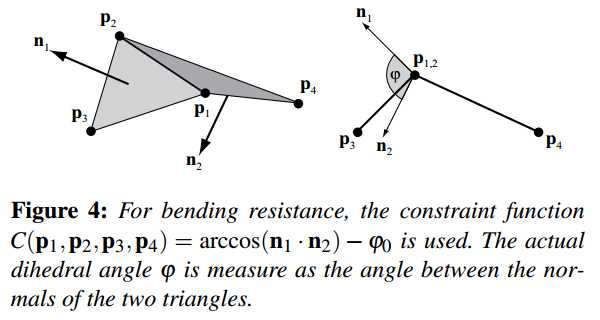
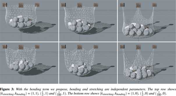
stiffness \(k_{bend}\) and type equality. The scalar \(\varphi_0\) is the initial dihedral angle between the two triangles and \(k_{bend}\) is a global user parameter defining the bending stiffness of the cloth (see Figure 4). The advantage of this bending term over adding a distance constraint between points \(\mathbf p_3\) and \(\mathbf p_4\) or over the bending term proposed by [GHDS03] is that it is independent of stretching. This is because the term is independent of edge lengths. This way, the user can specify cloth with low stretching stiffness but high bending resistance for instance (see Figure 3).
刚度为\(k_{bend}\) 类型为equality。标量\(\varphi_0\)是两个三角形的初始二面夹角。\(k_{bend}\)是用户定义的全局参数,表示布料的弯曲刚度(参见图4)。这个弯曲公式的优于在点\(\mathbf p_3\)和\(\mathbf p_4\)中添加距离约束,也优于[GHDS03]中提出的弯曲公式,公式的优点是independent of stretching。这是因为这个公式与边长无关。通过这种方式,用户可以指定低拉伸刚度,但抗弯强度更高的布料(见图3)。
Eqns. (10) and (11) define the projection for the stretching constraints. In the appendix A we derive the formulas to project the bending constraints.
公式(10)和公式(11)定义了拉伸约束的projection。在附录A中,我们给出了弯曲约束的projection公式。
4.2. Collision with Rigid Bodies
For collision handling with rigid bodies we proceed as described in Section 3.4. To get two-way interactions, we apply an impulse \(m_i \Delta \mathbf{p}_i / \Delta t\) to the rigid body at the contact point, each time vertex \(i\) is projected due to collision with that body. Testing only cloth vertices for collisions is not enough because small rigid bodies can fall through large cloth triangles. Therefore, collisions of the convex corners of rigid bodies against the cloth triangles are also tested.
对于与刚体的碰撞处理,我们按照第3.4节描述的进行。为了得到双向交互,我们在与刚体的接触点上应用一个脉冲\(m_i \Delta \mathbf{p}_i / \Delta t\),顶点\(i\)的投影操作每次都取决于和刚体的碰撞。仅仅测试布料顶点的碰撞是不够的,因为体型小的刚体可以穿过大的布料三角形。因此,刚体对布料网格的凸角的碰撞也需要测试。
4.3. Self Collision
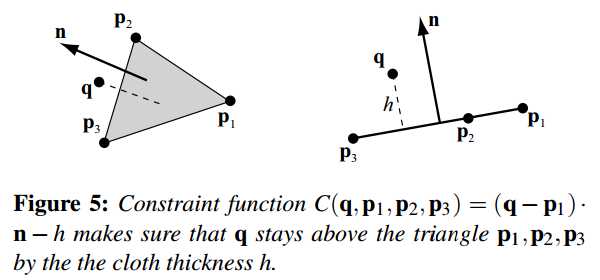
Assuming that the triangles all have about the same size, we use spatial hashing to find vertex triangle collisions [THM03]. If a vertex \(\mathbf q\) moves through a triangle \(\mathbf p_1\), \(\mathbf p_2\), \(\mathbf p_3\), we use the constraint function
假设所有的三角形的大小都近似相同,我们利用空间哈希查找三角形顶点碰撞(THM03)。如果顶点\(\mathbf q\)通过三角形\(\mathbf p_1\),\(\mathbf p_2\),\(\mathbf p_3\),我们使用约束函数
\[C(\mathbf q,\mathbf p_1, \mathbf p_2, \mathbf p_3) = (\mathbf q-\mathbf p_1) \cdot \frac{(\mathbf p_2 - \mathbf p_1)\times (\mathbf p_3 - \mathbf p_1)}{|(\mathbf p_2 - \mathbf p_1)\times (\mathbf p_3 - \mathbf p_1)|} -h \tag{12}\]
where \(h\) is the cloth thickness (see Figure 5). If the vertex enters from below with respect to the triangle normal, the constraint function has to be
\(h\)是布的厚度(见图5)。如果顶点从三角形背面沿着法线方向穿过,那么约束函数应该是
\[C(\mathbf q,\mathbf p_1, \mathbf p_2, \mathbf p_3) = (\mathbf q-\mathbf p_1) \cdot \frac{(\mathbf p_3 - \mathbf p_1)\times (\mathbf p_2 - \mathbf p_1)}{|(\mathbf p_3 - \mathbf p_1)\times (\mathbf p_2 - \mathbf p_1)|} -h \tag{13}\]
to keep the vertex on the original side. Projecting these constraints conserves linear and angular momentum which is essential for cloth self collision since it is an internal process. Figure 6 shows a rest state of a piece of cloth with self collisions. Testing continuous collisions is insufficient if cloth gets into a tangled state, so methods like the ones proposed by [BWK03] have to be applied.
来保持顶点在原来一侧。在投影的时候保持约束的线性和角动量守恒,是布料自碰撞的关键,因为自碰撞是一个内部过程。图6显示了一块布与自碰撞的静止状态。如果布料进入纠缠态,测试连续碰撞是不够的,所以应该使用诸如[BWK03]提出的方法。
4.4. Cloth Balloons
For closed triangle meshes, overpressure inside the mesh can easily be modeled (see Figure 7). We add an equality constraint concerning all \(N\) vertices of the mesh with constraint function
对于封闭的三角网格,网格内部的压力可以简单的建模。我们增加一个equality约束,关联了网格中所有\(N\)个顶点
\[C(\mathbf p_1, \ldots , \mathbf p_N) = \left(\sum^{n_{\text{triangles}}}_{i=1}(\mathbf p_{t^i_1} \times \mathbf p_{t^i_2}) \cdot \mathbf p_{t^i_3}\right) - k_{\text{pressure}}V_0 \tag{14}\]
and stiffness \(k=1\) to the set of constraints. Here \(t^i_1\),\(t^i_2\) and \(t^i_3\) are the three indices of the vertices belonging to triangle \(i\). The sum computes the actual volume of the closed mesh. It is compared against the original volume \(V_0\) times the overpressure factor \(k_{\text{pressure}}\). This constraint function yields the gradients
该约束刚度\(k=1\),将其添加到约束集中。这里\(t^i_1\)、\(t^i_2\)和\(t^i_3\)是三角形\(i\)的顶点索引。约束公式中,求和部分计算的结果为封闭网格的实际体积。该约束的含义就是将其与原体积\(V_0\)乘以压力因子\(k_{\text{pressure}}\)进行比较。这个约束函数产生梯度为
\[ \nabla_{\mathbf p_i}C = \sum_{j:t^i_1=i}(\mathbf p_{t^j_2} \times \mathbf p_{t^j_3}) + \sum_{j:t^i_2=i}(\mathbf p_{t^j_3} \times \mathbf p_{t^j_1}) + \sum_{j:t^i_3=i}(\mathbf p_{t^j_1} \times \mathbf p_{t^j_2}) \tag{15} \]
These gradients have to be scaled by the scaling factor given in Eq. (7) and weighted by the masses according to Eq. (9) to get the final projection offsets \(\Delta \mathbf p_i\).
这些梯度必须按公式(7)给出的比例因子进行缩放,并根据公式(9)进行加权,得到最终的投影偏移\(\Delta \mathbf p_i\)。
References
[THM03] TESCHNER M., HEIDELBERGER B., MüLLER M., POMERANERTS D., GROSS M.: Optimized spatial hashing for collision detection of deformable objects. Proc. Vision, Modeling, Visualization VMV 2003 (2003), 47–54
[BWK03] BARAFF D., WITKIN A., KASS M.: Untangling cloth. In Proceedings of the ACM SIGGRAPH (2003), pp. 862–870.