Acting under uncertainty
1. Summarizing uncertainty
In many domains, the agent’s knowledge can at best provide only a degree of belief in the relevant sentences. Our main tool for dealing with degrees of belief is probability theory.
The ontological commitments of logic and probability theory are the same – that the world is composed of facts that do or do not hold in any particular case;
The epistemological commitments of logic and probability theory are different: A logical agent believes each sentence to be true or false or has no opinion, whereas a probabilistic agent may have a numerical degree of belief between 0 (certainly false) and 1 (certainly true).
Probability statements are made with respect to a knowledge state, not with respect to the real world.
Uncertainty arises because of both laziness and ignorance. It is inescapable in complex, nondeterministic, or partially observable environments.
Probabilities express the agent’s inability to reach a definite decision regarding the truth of a sentence. Probabilities summarize the agent’s beliefs relative to the evidence.
2. Uncertainty and rational decisions
Outcome: An outcome is a completely specified states.
Utility theory: Says that every state has a degree of usefulness, or utility, to an agent and that the agent will prefer states with higher utility. We use utility theory to represent and reason with preferences.
To make a rational choice, an agent must first have preferences between the different possible outcomes of the various plans.
The utility of a state is relative to an agent, a utility function can account for any set of preferences.
Decision theory = probability theory + utility theory.
The principle of maximum expected utility (MEU): The fundamental idea of decision theory, says that an agent is rational if and only if it chooses the action that yields the highest expected utility, averaged over all the possible outcomes of the action.
An decision-theoretic agent, at an abstract level, is identical to the agent that maintain a belief state reflecting the history of percepts to date. The primary difference is that the decision-theoretic agents’ belief state represents not just the possibilities for world states but also their probabilities.
Decision theory combines the agent’s beliefs and desires, defining the best action as the one that maximizes expected utility.
Basic probability notation
1. What probabilities are about
Sample space (Ω): The set of all possible worlds (ω).
A possible world is defined to be an assignment of values to all of the random variables under consideration.
The possible worlds are mutually exclusive and exhaustive – two possible worlds cannot both be the case, and one possible world must be the case.

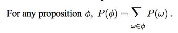
Events: A set of particular possible worlds that probabilistic assertion and queries are usually about. The set are always described by propositions For each proposition, the corresponding set contains just those possible worlds in which the proposition holds.
Basic probability statements include prior probabilities and conditional probabilities over simple and complex propositions.
Unconditional probabilities / Prior probabilities (“priors” for short): Degrees of belief in propositions in the absence of any other information. E.g. P(cavity)
Evidence: Some information that has already been revealed.
Conditional probability / posterior probability (“posterior” for short): P(event|evidence). e.g. P (cavity | toothache)
P(…|…) always means P((…)|(…)).
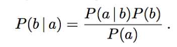
For any propositions a and b, we have,
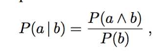
which holds whenever P(b) > 0.
The product rule: P(a∧b) = P(a|b)P(b).
2. The language of proposition in probability assertions
random variables: Variables in probability theory, their names begin with an uppercase letter. E.g. Total; Die1.
By convention, propositions of the form A=true are abbreviated simply as a, while A = false is abbreviated as ?a.
When no ambiguity is possible, it is common to use a value by itself to stand for the proposition that a particular variable has that value. E.g. sunny can stand for Weather = sunny.
Domain: The set of possible value that a random variable can take on.
Variable can have finite or infinite domains – either discrete or continuous.
For any variable with an ordered domain, inequalities are allowed.
Probability distribution: When we assume a predefined ordering on the domain of a random variable, we can write the probabilities of all the possible values as an abbreviation bold P.
e.g.
P(Wether = sunny) = 0.6, P(Wether = rain) = 0.1, P(Weather = cloudy) = 0.29, P(Weather = snow) = 0.01.
As an abbreviation: P(Weather) = <0.6, 0.1, 0.29, 0.01>.
The P notation is also used for conditional distribution: P(X|Y) gives the value of P(X=xi|Y=yi) for each possible i, j pair.
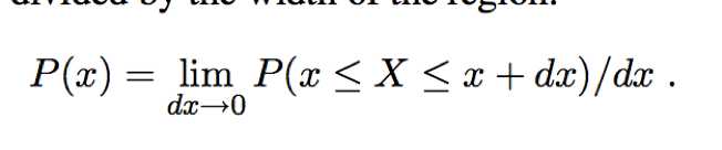
Probability density function (pdfs): For continuous variables, we can define the probability that a random variable takes on some value x as a parameterized function of x.
We write the probability density for a continuous random variable X at variable x as P(X=x) or just P(x);
e.g.
P(NoonTemp=x) = Uniform[18C, 26C](x)
Expresses the belief that the temperature at noon is distributed uniformly between 18C and 26C.
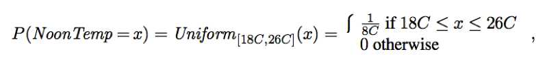
Notice that probabilities are unitless number, whereas density functions are measured with a unit.
(e.g.
1/8C is not a probability, it is a probability density. The probability that
NoonTemp is exactly 20.18C is zero because 20.18C is a region of width 0.)
Joint probability distribution: Notation for distribution on multiple variables.
e.g. P(Weather, Cavity) is a 4*2 table of probabilities of all combination of the values of Weather and Cavity.
We can mix variables with and without values.
e.g. P(sunny, Cavity) is a two-element vector giving the probabilities of a sunny day with a cavity and a sunny day with no cavity.
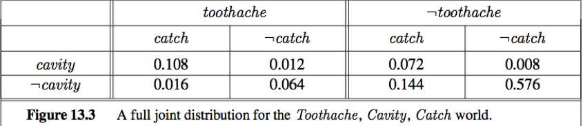
Full joint probability distribution: The joint distribution for all of the random variable, a probability model is completely determined by it.
e.g. if the variable are Cavity, Toothache and Weather, then the full joint distribution is given by P(Cavity, Toothache, Weather).
2. Probability axioms and their reasonableness
The inclusion-exclusion principle: P(a∨b) = P(a) + P(b) – P(a∧b)
Kolmogorov’s axioms:
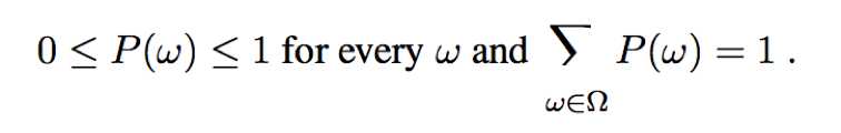
and
P(a∨b) = P(a) + P(b) – P(a∧b)
The axioms of probability constrain the possible assignments of probabilities to propositions. An agent that violates the axioms must behave irrationally in some cases.
Inference using full joint distribution
Probabilistic inference: The computation of posterior probabilities for query propositions given observed evidence.
The full joint probability distribution specifies the probability of each complete assignment of values to random variables. It is usually too large to create or use in its explicit form, but when it is available it can be used to answer queries simply by adding up entries for the possible worlds corresponding to the query propositions.
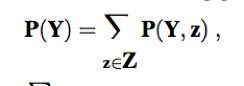
Marginalizatiion / summing out: The process of extract the distribution over some subset of variables or a single variable (to get the marginal probability), by summing up the probabilities for each possible value of the other variables, thereby taking them out of the equation.
e.g. The marginal probability of cavity is P(cavity) = 0.108+0.012+0.072+0.008
The general marginalization rule for any sets of variables Y and Z:
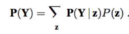
The conditioning rule:
Normalization constant (α): 1/P(evidence) can be viewed as a normalization constant for the distribution P(event | evidence), ensuring that it adds up to 1.
X (Cavitiy) is a single variable. Let E (Toothache) be the list of evidence variables, e be the list of observed values for them, Y (Catch) be the remaining unobserved variables. The query P(X|e) can be evaluated as:
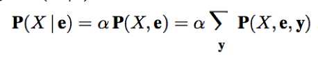
e.g.
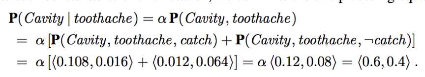
(We can calculate it even if we don’t know the value of P(toothache).)
Independence
Independence (a.k.a. Marginal independence / absolute independence):
Independence between propositions a and b can be written as: (all equivalent)
P(a|b) = P(a) or P(b|a) = P(b) or P(a∧b) = P(a)P(b).
Independence between variables X and Y can be written as:
P(X|Y) = P(X) or P(Y|X) = P(Y) or P(X, Y) = P(X)P(Y).
Independence assertions can dramatically reduce the amount of information necessary to specify the full joint distribution. If the complete set of variables can be divided into independent subsets, then the full joint distribution can be factored into separate joint distributions on those subsets.
Absolute independence between subsets of random variables allows the full joint distribution to be factored into smaller joint distributions, greatly reducing its complexity. Absolute independence seldom occurs in practice.
Bayes’ rule and its use
The Bayes’ rule:
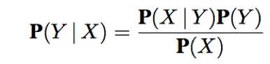
The Baye’s rule for multivalued variables: (representing a set of equations, each dealing with specific values of the variables)

The Baye’s rule conditionalized on some evidence e:
1. Applying Baye’s rule: the simple case
We perceive as evidence the effect of some unknown cause, and we would like to determine that cause. Apply Baye’s rule:
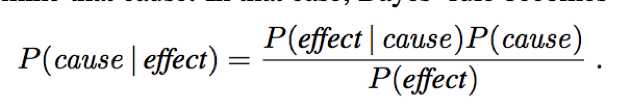
P(effect|cause) (e.g. P(symptoms|disease)) quantifies the relationship in the causal direction;
P(cause|effect) (e.g. P(disease|symptoms)) describes the diagnostic direction.
e.g.
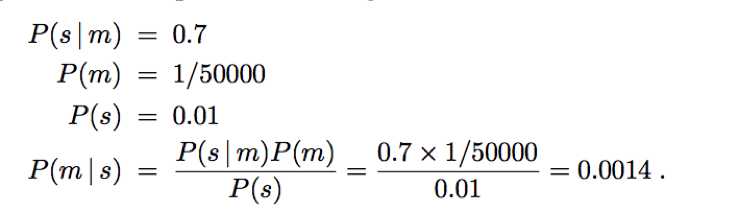
We can avoid assessing the prior probability of the evidence (P(s)) by instead computing a posterior probability for each value of the query variable (m and ?m) and then normalizing the result.

The general form of Bayes’ rule with normalization:
P(Y|X) = αP(X|Y)P(Y), where α is the normalization constant needed to make the entries in P(Y|X) sum to 1.
Bayes’ rule allows unknown probabilities to be computed from known conditional probabilities, usually in the causal direction. Applying Bayes’ rule with many pieces of evidence runs into the same scaling problems as does the full joint distribution.
2. Using Bayes’ rule: combining evidence
The general definition of conditional independence of two variable X and Y, given a third variable Z is:
P(X, Y|Z) = P(X|Z)P(Y|Z)
The equivalent forms can also be used:
P(X|Y, Z) = P(X|Z) and P(Y|X, Z) = P(Y|Z)
e.g.
assert conditional independence of the variables Toothache and Catch, given Cavity:
P(Toothache, Catch|Cavity) = P(Toothache|Cavity)P(Catch|Cavity).
Absolute independence assertions allow a decomposition of the full joint distribution into much smaller pieces, the same is true for conditional independence assertions.
Na?ve Bayes model: In which a single cause directly influences a number of effects, all of which are conditionally independent, given the cause. The full joint distribution can be written as
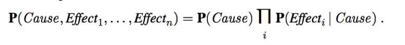
Conditional independence brought about by direct causal relationships in the domain might allow the full joint distribution to be factored into smaller, conditional distributions. The na?ve Bayes model assumes the conditional independence of all effect variables, given a single cause variable, and grow linearly with the number of effects.
The wumpus world revisited
A wumpus-world agent can calculate probabilities for unobserved aspects of the world, thereby improving on the decisions of a purely logical agent. Conditional independence makes these calculations tractable.