代码:
%% ------------------------------------------------------------------------
%% Output Info about this m-file
fprintf(‘\n***********************************************************\n‘);
fprintf(‘ <DSP using MATLAB> Problem 3.22 \n\n‘);
banner();
%% ------------------------------------------------------------------------
%% -------------------------------------------------------------------
%% 1 xa(t)=cos(20πt+θ) through A/D
%% -------------------------------------------------------------------
Ts = 0.05; % sample interval, 0.05s
Fs = 1/Ts; % Fs=20Hz
%theta = 0;
%theta = pi/6;
%theta = pi/4;
%theta = pi/3;
theta = pi/2;
n1_start = 0; n1_end = 20;
n1 = [n1_start:1:n1_end];
nTs = n1 * Ts; % [0, 1]s
x1 = cos(20*pi*nTs + theta * ones(1,length(n1))); % Digital signal
M = 500;
[X1, w] = dtft1(x1, n1, M);
magX1 = abs(X1); angX1 = angle(X1); realX1 = real(X1); imagX1 = imag(X1);
%% --------------------------------------------------------------------
%% START X(w)‘s mag ang real imag
%% --------------------------------------------------------------------
figure(‘NumberTitle‘, ‘off‘, ‘Name‘, sprintf(‘Problem 3.22 X1, theta/pi = %f‘, theta/pi));
set(gcf,‘Color‘,‘white‘);
subplot(2,1,1); plot(w/pi,magX1); grid on; %axis([-1,1,0,1.05]);
title(‘Magnitude Response‘);
xlabel(‘frequency in \pi units‘); ylabel(‘Magnitude |H|‘);
subplot(2,1,2); plot(w/pi, angX1/pi); grid on; %axis([-1,1,-1.05,1.05]);
title(‘Phase Response‘);
xlabel(‘frequency in \pi units‘); ylabel(‘Radians/\pi‘);
figure(‘NumberTitle‘, ‘off‘, ‘Name‘, sprintf(‘Problem 3.22 X1, theta/pi = %f‘, theta/pi));
set(gcf,‘Color‘,‘white‘);
subplot(2,1,1); plot(w/pi, realX1); grid on;
title(‘Real Part‘);
xlabel(‘frequency in \pi units‘); ylabel(‘Real‘);
subplot(2,1,2); plot(w/pi, imagX1); grid on;
title(‘Imaginary Part‘);
xlabel(‘frequency in \pi units‘); ylabel(‘Imaginary‘);
%% -------------------------------------------------------------------
%% END X‘s mag ang real imag
%% -------------------------------------------------------------------
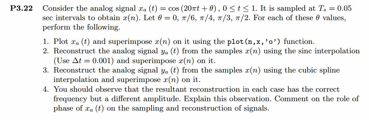
figure(‘NumberTitle‘, ‘off‘, ‘Name‘, sprintf(‘Problem 3.22 xa(n), theta/pi = %f and x1(n)‘, theta/pi));
na1 = 0:0.01:1;
xa1 = cos(20 * pi * na1 + theta * ones(1,length(na1)));
set(gcf, ‘Color‘, ‘white‘);
plot(1000*na1,xa1); grid on; %axis([0,1,0,1.5]);
title(‘x1(n) and xa(n)‘);
xlabel(‘t in msec.‘); ylabel(‘xa(t)‘); hold on;
plot(1000*nTs, x1, ‘o‘); hold off;
%% ------------------------------------------------------------
%% xa(t) reconstruction from x1(n)
%% ------------------------------------------------------------
Dt = 0.001; t = 0:Dt:1;
xa = x1 * sinc(Fs*(ones(length(n1),1)*t - nTs‘*ones(1,length(t)))) ;
figure(‘NumberTitle‘, ‘off‘, ‘Name‘, sprintf(‘Problem 3.22 Reconstructed From x1(n), theta/pi = %f‘, theta/pi));
set(gcf,‘Color‘,‘white‘);
%subplot(2,1,1);
stairs(t*1000,xa,‘r‘); grid on; %axis([0,1,0,1.5]); % Zero-Order-Hold
title(‘Reconstructed Signal from x1(n) using Zero-Order-Hold‘);
xlabel(‘t in msec.‘); ylabel(‘xa(t)‘); hold on;
%stem(nTs*1000, x1); gtext(‘ZOH‘); hold off;
plot(nTs*1000, x1, ‘o‘); gtext(‘ZOH‘); hold off;
figure(‘NumberTitle‘, ‘off‘, ‘Name‘, sprintf(‘Problem 3.22 Reconstructed From x1(n), theta/pi = %f‘, theta/pi));
set(gcf,‘Color‘,‘white‘);
%subplot(2,1,2);
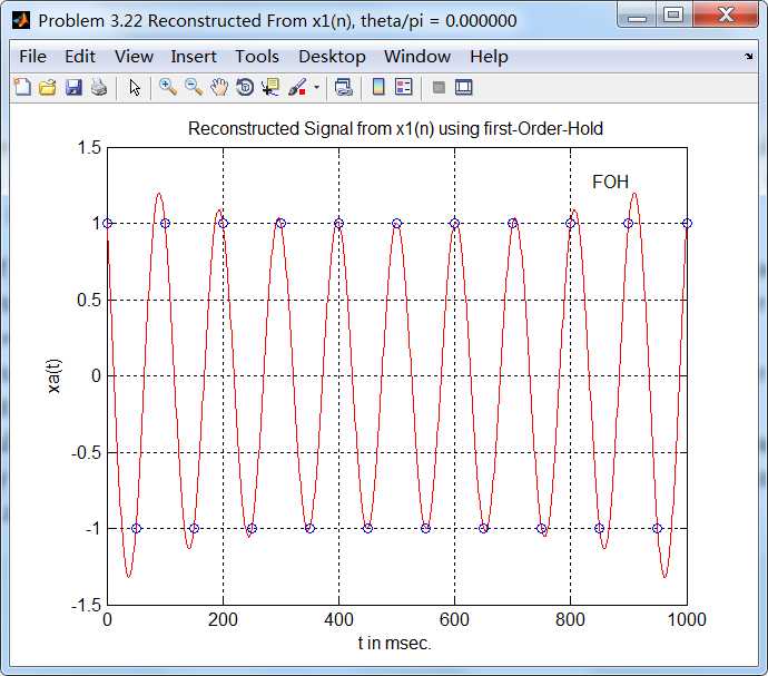
plot(t*1000,xa,‘r‘); grid on; %axis([0,1,0,1.5]); % first-Order-Hold
title(‘Reconstructed Signal from x1(n) using First-Order-Hold‘);
xlabel(‘t in msec.‘); ylabel(‘xa(t)‘); hold on;
plot(nTs*1000,x1,‘o‘); gtext(‘FOH‘); hold off;
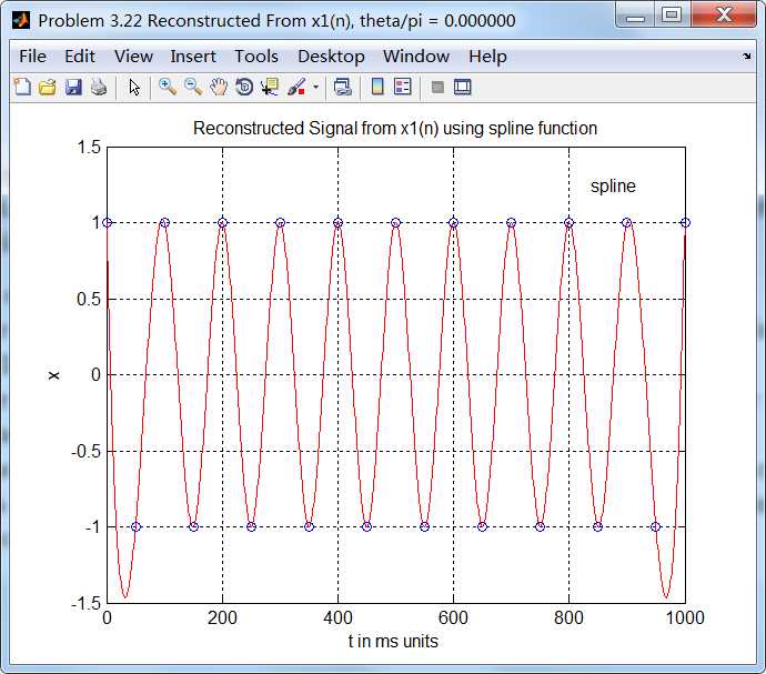
xa = spline(nTs, x1, t);
figure(‘NumberTitle‘, ‘off‘, ‘Name‘, sprintf(‘Problem 3.22 Reconstructed From x1(n), theta/pi = %f‘, theta/pi));
set(gcf,‘Color‘,‘white‘);
%subplot(2,1,1);
plot(1000*t, xa,‘r‘);
xlabel(‘t in ms units‘); ylabel(‘x‘);
title(sprintf(‘Reconstructed Signal from x1(n) using Spline function‘)); grid on; hold on;
plot(1000*nTs, x1,‘o‘); gtext(‘spline‘);
运行结果:
这里只看初相位为0的情况,原始模拟信号和采样信号(样点值圆圈标示):
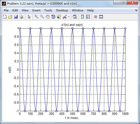
采样信号的谱,模拟角频率20π对应的数字角频率为π,如下图所示:
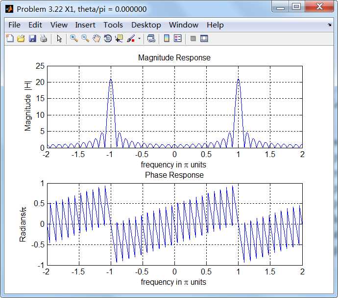
用采样信号重建原来模拟信号:
sinc方法,stairs函数画图
sinc方法,plot函数画图:
cubic方法
其他初相位的情况,这里不上图了。