第二节，TensorFlow 使用前馈神经网络实现手写数字识别

时间：2018-04-01 22:58:37 阅读：491 评论：0 收藏：0 [点我收藏+]

标签：alt art trunc val 学习 set 线性 margin lock

一感知器

感知器学习笔记：https://blog.csdn.net/liyuanbhu/article/details/51622695

感知器（Perceptron）是二分类的线性分类模型，其输入为实例的特征向量，输出为实例的类别，取+1和-1。这种算法的局限性很大：

只能将数据分为 2 类
数据必须是线性可分的

虽然有这些局限，但是感知器是 ANN 和 SVM 的基础，理解了感知器的原理，对学习ANN 和 SVM 会有帮助，所以还是值得花些时间的。

感知器可以表示为 f:Rⁿ -> {-1,+1}的映射函数，其中f的形式如下：

f(x) = sign(w.x+b)

其中w,b都是n维列向量，w表示权重，b表示偏置，w.x表示w和x的内积。感知器的训练过程其实就是求解w和b的过程，正确的w和b所构成的超平面

w.x + b=0恰好将两类数据点分割在这个平面的两侧。

二神经网络

今天，使用的神经网络就是由一个个类似感知器的神经元模型叠加拼接成的。目前常用的神经元包括S型神经元，ReLU神经元，tanh神经元，Softmax神

经元等等。

手写数字识别是目前在学习神经网络中普遍使用的案例。在这个案例中将的是简单的全连接网络实现手写数字识别，这个例子主要包括三个部分。

1.模型搭建

2.确定目标函数，设置损失和梯度值

3.选择算法，设置优化器选择合适的学习率更新权重和偏置。

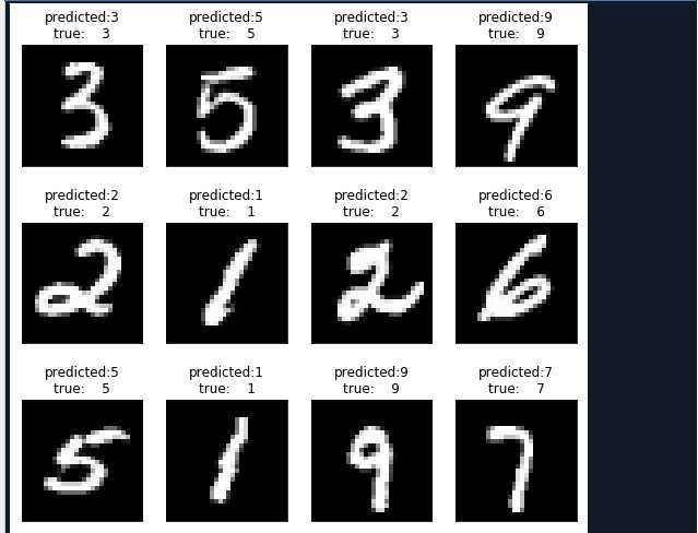
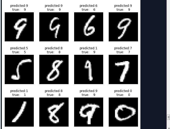
手写数字识别代码如下：

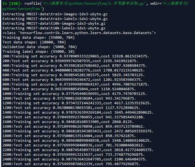
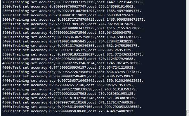
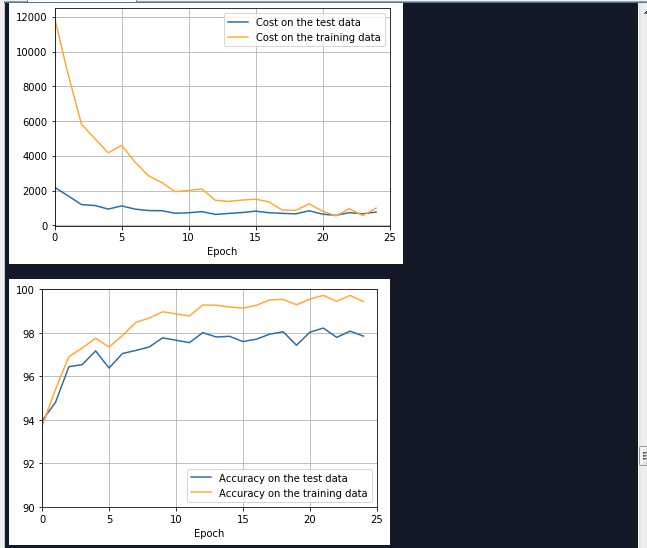
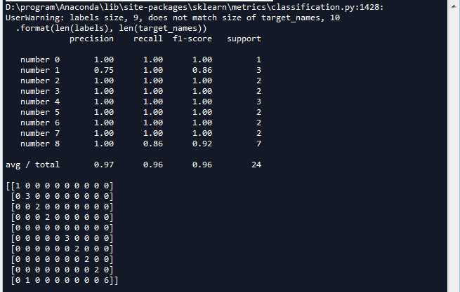
# -*- coding: utf-8 -*-
"""
Created on Sun Apr  1 19:16:15 2018

@author: Administrator
"""

‘‘‘
使用TnsorFlow实现手写数字识别
‘‘‘

import numpy as np
import matplotlib.pyplot as plt

#绘制训练集准确率，以及测试卷准确率曲线
def plot_overlay_accuracy(training_accuracy,test_accuaracy):
    ‘‘‘
    test_accuracy,training_accuracy:训练集测试集准确率
    ‘‘‘    
    #迭代次数
    num_epochs = len(test_accuaracy)
    
    fig = plt.figure()
    ax = fig.add_subplot(111)
    ax.plot(np.arange(0, num_epochs), 
            [accuracy*100.0 for accuracy in test_accuaracy], 
            color=‘#2A6EA6‘,
            label="Accuracy on the test data")
    ax.plot(np.arange(0, num_epochs), 
            [accuracy*100.0 for accuracy in training_accuracy], 
            color=‘#FFA933‘,
            label="Accuracy on the training data")
    ax.grid(True)
    ax.set_xlim([0, num_epochs])
    ax.set_xlabel(‘Epoch‘)
    ax.set_ylim([90, 100])
    plt.legend(loc="lower right")              #右小角
    plt.show()
    

#绘制训练集代价和测试卷代价函数曲线
def plot_overlay_cost(training_cost,test_cost):
    ‘‘‘
    test,reaining:训练集测试集代价  list类型  
    ‘‘‘    
    #迭代次数
    num_epochs = len(test_cost)
    
    fig = plt.figure()
    ax = fig.add_subplot(111)
    ax.plot(np.arange(0, num_epochs), 
            [cost for cost in test_cost], 
            color=‘#2A6EA6‘,
            label="Cost on the test data")
    ax.plot(np.arange(0, num_epochs), 
            [cost for cost in training_cost], 
            color=‘#FFA933‘,
            label="Cost on the training data")
    ax.grid(True)
    ax.set_xlim([0, num_epochs])
    ax.set_xlabel(‘Epoch‘)
    #ax.set_ylim([0, 0.75])
    plt.legend(loc="upper right")
    plt.show()
    
from sklearn.metrics import classification_report
from sklearn.metrics import confusion_matrix
‘‘‘
打印图片
images：list或者tuple，每一个元素对应一张图片
title：list或者tuple，每一个元素对应一张图片的标题
h:高度的像素数
w:宽度像素数
n_row：输出行数
n_col：输出列数
‘‘‘
def plot_gallery(images,title,h,w,n_row=3,n_col=4):
    #指定整个绘图对象的宽度和高度
    plt.figure(figsize=(1.8*n_col,2.4*n_row))
    plt.subplots_adjust(bottom=0,left=.01,right=.99,top=.90,hspace=.35)
    #绘制每个子图
    for i in range(n_row*n_col):
        #第i+1个子窗口 默认从1开始编号
        plt.subplot(n_row,n_col,i+1)
        #显示图片 传入height*width矩阵 https://blog.csdn.net/Eastmount/article/details/73392106?locationNum=5&fps=1
        plt.imshow(images[i].reshape((h,w)),cmap=plt.cm.gray)  #cmap Colormap 灰度 
        #设置标题
        plt.title(title[i],size=12)
        plt.xticks(())
        plt.yticks(())
        
‘‘‘
打印第i个测试样本对应的标题
Y_pred：测试集预测结果集合 (分类标签集合)
Y_test: 测试集真实结果集合 (分类标签集合)
target_names:分类每个标签对应的名称
i:第i个样本
‘‘‘
def title(Y_pred,Y_test,target_names,i):
    pred_name = target_names[Y_pred[i]].rsplit(‘ ‘,1)[-1]
    true_name = target_names[Y_test[i]].rsplit(‘ ‘,1)[-1]
    return ‘predicted:%s\ntrue:    %s‘ %(pred_name,true_name)




import tensorflow as tf



#设置tensorflow对GPU使用按需分配
config = tf.ConfigProto()
config.gpu_options.allow_growth = True

sess = tf.InteractiveSession(config=config)

‘‘‘
一 导入数据
‘‘‘
from tensorflow.examples.tutorials.mnist import input_data

mnist = input_data.read_data_sets(‘MNIST-data‘,one_hot=True)

print(type(mnist)) #<class ‘tensorflow.contrib.learn.python.learn.datasets.base.Datasets‘>

print(‘Training data shape:‘,mnist.train.images.shape)           #Training data shape: (55000, 784)
print(‘Test data shape:‘,mnist.test.images.shape)                #Test data shape: (10000, 784)
print(‘Validation data shape:‘,mnist.validation.images.shape)    #Validation data shape: (5000, 784)
print(‘Training label shape:‘,mnist.train.labels.shape)          #Training label shape: (55000, 10)

‘‘‘
二 搭建前馈神经网络模型 搭建一个包含输入层分别为 784,1024,10个神经元的神经网络
‘‘‘

#初始化权值和偏重
def weight_variable(shape):
    #使用正太分布初始化权值
    initial = tf.truncated_normal(shape,stddev=0.1)    #标准差为0.1
    return tf.Variable(initial)

def bias_variable(shape):
    initial = tf.constant(0.1,shape=shape)
    return tf.Variable(initial)




#input layer
x_ = tf.placeholder(tf.float32,shape=[None,784])
y_ = tf.placeholder(tf.float32,shape=[None,10])


#隐藏层
w_h = weight_variable([784,1024])
b_h = bias_variable([1024])
hidden = tf.nn.relu(tf.matmul(x_,w_h) + b_h)

#输出层
w_o = weight_variable([1024,10])
b_o = bias_variable([10])
output = tf.nn.softmax(tf.matmul(hidden,w_o) + b_o)


‘‘‘
三 设置对数似然损失函数
‘‘‘
#代价函数 J =-(Σy.logaL)/n    .表示逐元素乘
cost = -tf.reduce_sum(y_*tf.log(output))


‘‘‘
四 求解
‘‘‘
train = tf.train.AdamOptimizer(0.001).minimize(cost)

#预测结果评估
#tf.argmax(output,1)  按行统计最大值得索引
correct = tf.equal(tf.argmax(output,1),tf.argmax(y_,1))       #返回一个数组 表示统计预测正确或者错误 
accuracy = tf.reduce_mean(tf.cast(correct,tf.float32))   #求准确率


#创建list 保存每一迭代的结果
training_accuracy_list = []
test_accuracy_list = []
training_cost_list=[]
test_cost_list=[]


#使用会话执行图
sess.run(tf.global_variables_initializer())   #初始化变量
#开始迭代 使用Adam优化的随机梯度下降法
for i in range(5000):
    x_batch,y_batch = mnist.train.next_batch(batch_size = 64)   
    #开始训练
    train.run(feed_dict={x_:x_batch,y_:y_batch})   
    if (i+1)%200 == 0:
         #输出训练集准确率
        #training_accuracy = accuracy.eval(feed_dict={x_:mnist.train.images,y_:mnist.train.labels})
        training_accuracy,training_cost = sess.run([accuracy,cost],feed_dict={x_:mnist.train.images,y_:mnist.train.labels})
        training_accuracy_list.append(training_accuracy)
        training_cost_list.append(training_cost)        
        print(‘{0}:Training set accuracy {1},cost {2}.‘.format(i+1,training_accuracy,training_cost))
        #输出测试机准确率   
        #test_accuracy = accuracy.eval(feed_dict={x_:mnist.test.images,y_:mnist.test.labels})
        test_accuracy,test_cost = sess.run([accuracy,cost],feed_dict={x_:mnist.test.images,y_:mnist.test.labels})
        test_accuracy_list.append(test_accuracy)
        test_cost_list.append(test_cost) 
        print(‘{0}:Test set accuracy {1},cost {2}.‘.format(i+1,test_accuracy,test_cost))   
#绘制曲线图    
plot_overlay_cost(training_cost_list,test_cost_list)
plot_overlay_accuracy(training_accuracy_list,test_accuracy_list)



#取24个样本，可视化显示预测效果
x_batch,y_batch = mnist.test.next_batch(batch_size = 24)   
#获取x_batch图像对象的数字标签
y_test = np.argmax(y_batch,1)
#获取预测结果
y_pred = np.argmax(output.eval(feed_dict={x_:x_batch,y_:y_batch}),1)

#显示与分类标签0-9对应的名词
target_names = [‘number 0‘,‘number 1‘,‘number 2‘,‘number 3‘,‘number 4‘,‘number 5‘,‘number 6‘,‘number 7‘,‘number 8‘,‘number 9‘]
#需要测试的真实的标签和预测作为比较 显示主要的分类指标，返回每个类标签的精确、召回率及F1值
print(classification_report(y_test,y_pred,target_names = target_names))
#建立一个n*n 分别对应每一组真实的和预测的值 用于呈现一种可视化效果
print(confusion_matrix(y_test,y_pred,labels = range(len(target_names))))

#标题 
prediction_titles = [title(y_pred,y_test,target_names,i) for i in range(y_pred.shape[0])]
#打印图片
plot_gallery(x_batch,prediction_titles,28,28,6,4)
plt.show()