学习GLM的时候在网上找不到比较通俗易懂的教程。这里以一个实例应用来介绍GLM。
We used a Bayesian generalized linear model (GLM) to assign every gene to one or more cell populations, as previously described (Zeisel et al., 2015).
在单细胞RNA-seq的分析中,可以用GLM来寻找marker。
贝叶斯 + 广义 + 线性回归
线性回归:这个最基础,大部分人应该都知道。为什么找marker问题可以转化为线性回归问题?我们可以把每一个基因的表达当作自变量,把最终的类别作为因变量,拟合线性模型,然后根据系数的分布来得到marker。
广义:因变量(响应变量)可以服从多种分布(思考:为什么下文要用负二项分布);
贝叶斯:是一种新的思维方式,所有的系数都有自己的分布。
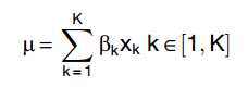
The GLM models the measured gene expression of a cell as realizations of a Negative Binomial probability distribution whose mean is determined by a linear combination of K predictors xi with coefficient bi.
For each cell, the outcome and predictors are known and the aim is to determine the posterior probability distributions of the coefficients.
As predictors, we use a continuous Baseline predictor and a categorical Cell Type predictor. The Baseline predictor value is the cell’s molecule count normalized to the average molecule count of all cells and takes account of the fact that we expect every gene to have a baseline expression proportional to the total number of expressed molecules within a particular cell. While the Cell Type predictor is set to 1 for the cluster BackSPIN assignation of the cell, and 0 for the other classes. From the definition of the model it follows that the coefficient bk for a Cell Type predictor xk can be interpreted as the additional number of molecules of a particular gene that are present as a result of the cell being of cell type k. A more detailed description of the model, including explanation of the prior probabilities used for the fitting as well as the full source code of the model, is provided elsewhere (Zeisel et al., 2015). The Stan (http://mc-stan.org) source is copied below for completeness:
data {
int < lower = 0 > N; # number of outcomes
int < lower = 0 > K; # number of predictors
matrix < lower = 0 > [N,K] x; # predictor matrix
int y[N]; # outcomes
}
parameters {
vector < lower = 1 > [K] beta; # coefficients
real < lower = 0.001 > r; # overdispersion
}
model {
vector < lower = 0.001 > [N] mu;
vector < lower = 1.001 > [N] rv;
# priors
r !cauchy(0, 1);
beta !pareto(1, 1.5);
# vectorize the overdispersion
for (n in 1:N) {
rv[n] < - square(r + 1) - 1;
}
# regression
mu < - x * (beta - 1) + 0.001;
y !neg_binomial(mu ./ rv, 1 / rv[1]);
}
To determine which genes are higher than basal expression in each population we compared the posterior probability distributions of the Baseline coefficient and the Cell Type coefficient. A gene was considered as marking a cell population if (1) its cell-typespecific coefficient exceeded the Baseline coefficient with 99.8% (95% for the mouse adult) posterior probability, and (2) the median of its posterior distribution did not fall below a threshold q set to 35% of the median posterior probability of the highest expressing group, and (3) the median of the highest-expressing cell type was greater than 0.4. For every gene this corresponds to a binary pattern (0 if the conditions are not met and 1 if they are), and genes can therefore be grouped according to their binarized expression patterns.
We use those binarized patterns to call transcription factor specificity. Our definition of a transcription factor gene was based of annotations provided by the merged annotation of PANTHER GO (Mi et al., 2013) and FANTOM5 (Okazaki et al., 2002), this list was further curated and missing genes and occasional misannotations corrected.
The feature selection procedure is based on the largest difference between the observed coefficient of variation (CV) and the predicted CV (estimated by a non-linear noise model learned from the data) See Figure S1C. In particular, Support Vector Regression (SVR, Smola and Vapnik, 1997) was used for this purpose (scikit-learn python implementation, default parameters with gamma = 0.06; Pedregosa et al., 2011).
特征选取:寻找观察CV值和预测CV值之间的最大差异。
SVR支持向量回归
Similarities between clusters within a species were summarized using a Pearson’s correlation coefficient calculated on the binarized matrix (Figures 1C and 1D).