标签:mini and instead ice should multi parallel paper class
Given \(N\) data samples in \(n\) dimensional space, i.e., \(Y \in R^{n\times N}\), the task is to compute the dictionary \(D\in R^{n\times K}\) and sparse component \(X\in R^{K\times N}\). Using the Frobenius norm, the task is summarized as the following optimization problem:

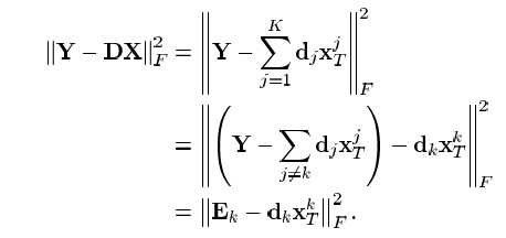
which is equivalent to

[Attention]
(1) If our aim is just the minimization of the first line shown above, the explicit solution is just the SVD of \(Y\), from which we can obtain \(d_j\) and \(x_T^j (j=1,\cdots,K)\). However this will not lead to a sparse \(x_T^j\).
(2) The idea here is to use the last line incremently, i.e., from \(k=1\) to \(K\). When optimizing \(d_k\) and \(x^k_T\), we fix other columns of \(D\) and rows of \(X\). In this way, we elminate the summation in the first line. Thereby, we can further apply the following sparse-holding technique.
(3) Direct using SVD of \(E_k\) to obtain \(d_k\) and \(x^k\) will definitely destroy the existing sparsity of \(x^k\), thus is unfavorable. A remedy is to only consider the nonzero element of \(x^k\), this is equivalent to a selection matrix defined by
\(\Omega_k\), the \(k\) here refer to the recursive procedure.
The effect of \(\Omega_k\) to \(x_k\) is just the selection of nonzero elements of \(x^k\). For example, if \(x=[1, 0, 2, 0, 3]\), then \(\Omega=[e_1,e_3,e_4]\in R^{5\times 3}\). So we can check that \(x\Omega=[1,2,3]\).
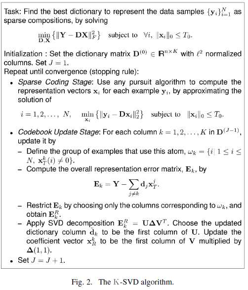
So instead of application of SVD to \(E_k\), in \(k-SVD\) we apply SVD to \(E_k^R:=E_k\Omega_k\). That is we optimize

and this time it can be done directly via SVD. We define the solution for \(d_k\) as the first column of \(U\) and the coefficient vector \(x_R^k\) as the first column of \(V\) multiplied by \(\sigma(1,1)\).
[Attention]
(1) There is a mistake in equation (22) in the original paper. The index \(i\) should in \(1\leq i\leq N\) rather than \(K\).
(2) Also when updating \(d_2\) and \(x^2\), we use the updated \(d_1\) and \(x^1\). That is to say, K-SVD works in a manner similar to G-S iteration.
(3) The original paper also says that you can also work in a parallel manner. That is to say update \(d_2\) and \(x^2\) using the same \(X\). But my question is how to do with \(d_1\)? Do we use the updated or the original one? The answer is left to the reader. You can compare it in the computer simulation.
The complete algorithm is shown below:(Notice in each loop, first compute sparse component \(X\), then sweep from \(k=1\) to \(K\) to obtain \(D\) and \(X\), then goes to the next iteration.)

Any comments are welcome. Tks.
标签:mini and instead ice should multi parallel paper class
原文地址:https://www.cnblogs.com/mathlife/p/9058392.html