标签：2.3   amp   his   欧拉   ESS   nts   检验   完美   res   

T distribution

定义

在概率论和统计学中，学生t-分布（t-distribution），可简称为t分布，用于根据小样本来估计 呈正态分布且方差未知的总体的均值。如果总体方差已知(例如在样本数量足够多时)，则应该用正态分布来估计总体均值。

In probability and statistics, Student‘s t-distribution (or simply the t-distribution) is any member of a family of continuous probability distributions that arises when estimating the mean of a normally distributed population in situations where the sample size is small and population standard deviation is unknown.

If we take a sample of n observations from a normal distribution, then the t-distribution with \(\displaystyle \nu =n-1\) degrees of freedom can be defined as the distribution of the location of the sample mean relative to the true mean, divided by the sample standard deviation, after multiplying by the standardizing term \(\displaystyle \sqrt {n}\). In this way, the t-distribution can be used to construct a confidence interval for the true mean.

概率密度函数(pdf)

\(f(t)=\frac{\displaystyle \Gamma(\frac{\nu+1}{2})}{\displaystyle \sqrt{\nu\pi}\cdot\Gamma(\frac {\nu} {2})} \Large \left(1+\frac{t^2}{\nu}\right)^{-\frac{\nu+1}{2}}\),where \(\displaystyle \nu\) is the number of degrees of freedom and \(\displaystyle \Gamma\) is the gamma function.

特点

t分布曲线形态与n(确切地说与自由度df)大小有关。与标准正态分布曲线相比，自由度df越小，t分布曲线愈平坦，曲线中间愈低，曲线双侧尾部翘得愈高；自由度df愈大，t分布曲线愈接近正态分布曲线，当自由度df->∞时，t分布曲线为标准正态分布曲线。

The t-distribution is symmetric and bell-shaped, like the normal distribution, but has heavier tails, meaning that it is more prone to producing values that fall far from its mean. This makes it useful for understanding the statistical behavior of certain types of ratios of random quantities, in which variation in the denominator is amplified and may produce outlying values when the denominator of the ratio falls close to zero. The Student‘s t-distribution is a special case of the generalised hyperbolic distribution.

作用

在概率论和统计学中，t-分布 经常应用在 对正态分布的总体的均值 进行估计。t检验改进了Z检验，不论样本数量大或小皆可应用。在样本数量大(超过120)时，可以应用Z检验，但Z检验用在小的样本会产生很大的误差，因此样本很小的情况下得改用t检验。

The t-distribution plays a role in a number of widely used statistical analyses, including Student‘s t-test for assessing the statistical significance of the difference between two sample means, the construction of confidence intervals for the difference between two population means, and in linear regression analysis. The Student‘s t-distribution also arises in the Bayesian analysis of data from a normal family.

t分布的产生

Let X1, ..., Xn be independent and identically distributed as N(μ, σ2), i.e. this is a sample of size n from a normally distributed population with expected mean value μ and variance σ2.

Let \(\overline X = \frac 1 n \displaystyle\sum_{i=1}^n X_i\) be the sample mean,Let \(S^2=\frac{1}{n-1}\displaystyle\sum_{i=1}^n(X_i-\overline X)^2\) be the(Bessel-corrected)sample variance.Then the random variable \(\frac{\overline X - \mu}{\frac {\sigma} {\sqrt n}}\) has a standard normal distribution(i.e. normal with expected value 0 and variance 1),and the random variable \(\frac{\overline X - \mu}{\frac{S}{\sqrt n}}\) (where S has been substituted for \(\sigma\))has a t distribution with n-1 degrees of freedom.

t分布置信区间的计算

Suppose the number A is so chosen that \(Pr(-A<T<A)=0.9\),when T has a t-distribution with n-1 degrees of freedom. By symmetry, this is the same as saying that A satisfies \(Pr(T<A)=0.95\),so A is the "95th percentile" of this probability distribution, or \(A=t_{(0.05,n-1)}\).Then \(\displaystyle Pr\left( -A < \frac{\overline X_n-\mu}{\frac {S_n}{\sqrt n}}<A \right)=0.9 => Pr\left( \overline X_n-A\cdot \frac{S_n}{\sqrt n}<\mu<\overline X_n+A\cdot \frac{S_n}{\sqrt n}\right)=0.9\).Therefore, the interval whose endpoints are \(\overline X_n \pm A\cdot \frac{S_n}{\sqrt n}\). It is a 90% confidence interval for \(\mu\).Therefore, if we find the mean of a set of observations that we can reasonably expect to have normal distribution,we can use the t-distribution to examine whether the confidence limits on that mean include some theoretically predicted value-such as the value predicted on a null hypothesis.

例1

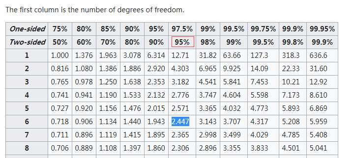
7 patients‘ blood pressure have been measured after having been given a new drug for 3 months.they had blood pressure increases of 1.5,2.9,0.9,3.9,3.2,2.1 and 1.9.Construct a 95% confidence interval for the true expected blood pressure increases for all patients in a population.

样本容量：n=7,

样本均值：\(\overline X=\frac{1.5+2.9+0.9+3.9+3.2+2.1+1.9}{7}=2.34\)

样本方差: \(S=\frac{(1.5-2.34)^2+(2.9-2.34)^2+(0.9-2.34^2)+(3.9-2.34^2)+(3.2-2.34)^2+(2.1-2.34)^2+(1.9-2.34)^2}{7-1}=1.04\)

查找t-table，自由度为6的95%的双侧T值为2.447

那么，置信区间的端点是\(2.34\pm2.447\cdot\frac{1.04}{\sqrt 7}=2.34\pm0.9618\)

自由度

统计学上，自由度是指当以样本的统计量来估计总体的参数时，样本中独立或能自由变化的数据的个数，称为该统计量的自由度。

自由度的解释：

1. 若存在两个变量a,b,且条件是a+b=1,显然，我们只要知道其中一个数(a),另一个数(b=1-a)会依赖a的值变化而变化，所以这组数的自由度为1
2. 估计总体的平均数(\(\mu\))时，由于样本中的n个数都是相互独立的，任一个尚未抽出的数都不受已抽出任何数值的影响，所以自由度为n。
3. 估计总体的方差(\(\sigma^2\))时所使用的统计量是样本的方差\(S^2\)，而\(S^2\)必须用到样本平均数\(\overline X\)来计算。在抽样完成后\(\overline X\)已确定，所以大小为n的样本中只要n-1个数确定了，第n个数的值就只有一个能使样本符合\(\overline X\)的数值。也就是说，样本中只有n-1个数可以自由变化，只要确定了这n-1个数，方差\(S^2\)也就确定了。这里，平均数\(\overline X\)就相当于一个限制条件，由于加了这个限制条件，样本方差\(S^2\)的自由度为n-1。

有一个有4个数据(n=4)的样本，其平均值m等于5，即受到m=5的条件限制，在自由确定4、2、5三个数据后， 第四个数据只能是9，否则\(m\neq5\)。因而这里的自由度df=n-1=4-1=3。推而广之，任何统计量的自由度df=n-k(k为限制条件的个数)。

伽马函数

In mathematics, the gamma function (represented by \(\Gamma\),the capital Greek alphabet letter gamma) is an extension of the factorial function, with its argument shifted down by 1, to real and complex numbers. If n is a positive integer,\(\Gamma(n)=(n-1)!\)

伽马函数产生背景

1728年，哥德巴赫在考虑数列插值的问题，通俗的说就是把数列的通项公式定义从整数集合延拓到实数集合，例如数列1,4,9,16.....可以用通项公式n2自然的表达，即便 n 为实数的时候，这个通项公式也是良好定义的。直观的说也就是可以找到一条平滑的曲线y=x2通过所有的整数点(n,n2),从而可以把定义在整数集上的公式延拓到实数集合。一天哥德巴赫开始处理阶乘序列1,2,6,24,120,720,...,我们可以计算2!,3!,是否可以计算2.5!呢?我们把最初的一些(n,n!)的点画在坐标轴上，确实可以看到，容易画出一条通过这些点的平滑曲线。但是哥德巴赫无法解决阶乘往实数集上延拓的这个问题，于是写信请教尼古拉斯·伯努利和他的弟弟丹尼尔·伯努利，由于欧拉当时和丹尼尔·伯努利在一块，他也因此得知了这个问题。而欧拉于1729 年完美地解决了这个问题，由此导致了伽玛函数的诞生，当时欧拉只有22岁。

小马哥课堂-统计学-t分布

标签：2.3   amp   his   欧拉   ESS   nts   检验   完美   res   

原文地址：https://www.cnblogs.com/black-mamba/p/9493694.html