标签:example nis point fixed index gravity sim version run
Chapter 1. Points and Lines (已看)
Chapter 2. Geometry Snippets (已看)
Chapter 3. Trigonometry Snippets (已看)
Chapter 4. Vector Operations (已看)
Chapter 5. Matrix Operations (已看)
Chapter 6. Transformations (已看)
Chapter 7. Unit Convensions (已看)
Chapter 8. Motion in One Dimension (已看)
Chapter 9. Derivative Approach to Motion in One Dimension (已看)
Chapter 10. Motion in Two and Three Dimensions (已看)
Chapter 11. Newton‘s Laws (已看)
Chapter 12. Energy (已看)
Chapter 13. Momentum and Collisions
Chapter 1. Points and Lines
The Point Defined

// Some various data types which can be used to store points
// 1. an array of floats. The advantage lies in speed, ease, and low
//  memory cost
float 3dPoint[3];

// 2. a structure holding 3 floats. The advantage lies in the
// ability to overload operators and define functions
struct 3dPoint {
    float x, y, z;
    // The overloaded addtion operator
    3dPoint operator+(const 3dPoint & P2) const {
        3dPoint temp = {
            this->x + P2.x,
            this->y + P2.y,
            this->z + p2.z
        };

        return temp;
    }
};

3dPoint A, B, C;
C = A + B;l
The Line Defined
Properties of Lines

// purpose: calculate the slope of a line given 2 points
// input: P1 - an array of 2 floats representing point 1
//          P2 -  an array of 2 floats representing point 2
// output: the slope between our 2 points
float slopeBetweenPoints(float * P1, float * P2) {
    return (P2[1] - P1[1]) / (P2[0] - P1[0]);
}

// purpose: to determine the slope of the line perpendicular to
// ourselves
// input: slope - the slope of our line
// output: the slope of a line perpendicular to us
float perpSlope(float slope) {
    return -1 / slope;
}

// purpose: to determine whether two lines are perpendicular
// input: slope1 - the slope of the first line
//           slope2 - the slope of our second line
// output: true if the lines are perpendicular, else false
bool arePerp(float slope1, float slope2) {
    if (slope1 * slope2 == -1) {
        return true;

    return false;
}
For any line in standard form, Ax + By = C, the slope m = -A / B;
Slope-intercept form: y = mx + b;
Point-slope form: (y - y1) = m(x - x1), where (x1, y1) is a point on the line
Applications in Collision Detection
Self-Assessment Solutions
Chapter 2. Geometry Snippets
Distance Between Points
Parabolas
A Parabola with a Vertical Axis y = a(x - h)2 + k, with vertex (h, k) and axis of symmetry x = h
A Parabola with a Horizontal Axis x = a(y - k)2 + h, with vertex (h, k) and axis of symmetry y = k
Circles and Spheres

struct circle {
    float center[2];
    float radius;
};

struct sphere {
    float center[3];
    float radius;
};
The Equation of a Circle (x - h)2 + (y - k)2 = r2 where the center is (h, k) and the radius is r
Equation of a Circle Centered at the Origin x2 + y2 = r2 where the center is (0,0) and the radius is r
Equation of a Sphere (x - h)2 + (y - k)2 + (z - l)2 = r2 where the center is (h,k,l) and the radius is r
Equation of a Sphere Centered at the Origin x2 + y2 + z2 where the center is (0, 0, 0) and the radius is r
Applications in Collision Detection
Visualization Experience: Collision Detection
Self-Assessment Solutions
Chapter 3. Trigonometry Snippets
Degrees Versus Radians
Trigonometric Functions

// purpose: to calculate the angle between 2 objects in 2D space
// input: P1 - the location of the first object
//           P2 - the location of the second object
// output: the angle between the objects in degrees
float calcAngle2D(float * P1, float * P2) {
    // Calculate our angle
    float angle = (float)atan((P2[1] - P1[1]) / (P2[0] - P1[0])) * RadToDeg;
    // In the event that the angle is in the first quardrant
    if (P2[1] < P1[1] && P2[0] > P1[0])
        return ang;
    // In the event of second or third quadrant
    else if ((P2[1] < P1[1] && P2[0] < P1[0]) || (P2[1] > P1[1] && P2[0] < P1[0]))
        return arg + 180;
    // If none of the above, it must be in the fourth
    else
        return arg + 360;
}
Trigonometric Identities
Unit Circle Identity cos2a + sin2a = 1
Tangent and Cotangent tan a = sin a / cos a cot a = cos a / sin a
Negative Angles sin(-a) = -sin a cos(-a) = cos a tan(-a) = -tan a
Sum and Difference Identities for Sine sin(a1 + a2) = sina1cosa2 + cosa1sina2 sin(a1 - a2) = sina1cosa2 - cosa1sina2
Sum and Difference Identities for Cosine cos(a1 + a2) = cosa1cosa2 - sina1sina2 cos(a1 - a2) = cosa1cosa2 + sina1sina2
Using Math Libraries in C++
Self-Assessment Solutions
Chapter 4. Vector Operations
Vector Versus Scalar
Vector Versus Scalar Scalar = magnitude only Vector = magnitude + direction
Displacement is the vector version of distance, and velocity is the vector version of speed
Polar Coordinates Versus Cartesian Coordinates
Vector Addition and Subtraction
Scalar Multiplication
Dot Product
The Dot Product in 2D A?B = a1b1 + a2b2 for any 2D vectors A = [a1 b1] and B = [b1 b2].
The Dot Product in 3D A?B = a1b1 + a2b2 + a3b3 for any 3D vectors A = [a1 b1 c1] and B = [b1 b2 b3]
Perpendicular Check if A?B = 0, A perp B
Positive or Negative Dot Product if A?B < 0 (negative), q > 90 if A?B > 0 (positive), q < 90 where q is the angle between vectors A and B
Cross Product
Cross Product A x B = [a2b3 - a3b2 a3b1 - a1b3 a1b2 - a2b1] for any two vectors A = [a1 a2 a3] and B = [b1 b2 b3]
Perpendicular Vectors A x B is perpendicular to both vectors A and B
Surface Normal Surface normal = (AXB)unit = AXB / ||AXB||
Visualization Experience
Self-Assessment Solutions
Chapter 5. Matrix Operations
Equal Matrices
Equal Matrices Two matrices are equal if 1.Both matrices have equal dimensions 2. All corresponding entries are equal
Matrix Addition and Subtraction
Scalar Multiplication
Matrix Multiplication
Transpose
Visualization Experience
Self-Assessment Solutions
Chapter 6. Transformations
Transformations is really just a fancy word for moving objects around in your world.It encompass movement such as forward and backward or up and down motion,scaling objects larger or smaller, and even rotating objects.
The term affine is indicates that the essential shape of the object being moved is preserved.
Translation
The fancy name for moving objects in directions is translation
2D Translation by Addition (x‘ y‘)t = (x y)t + (dx dy)t
3D Translation by Addition (x‘ y‘ z‘)t = (x y z)t + (dx dy dz)t
2D Translation by Multiplication  where dx = change in x and dy = change in y.
Notice that the old point and the new point have an extra 1 on the end. It‘s not actually part of the point, but it needs to tag along for the matrix math to work

Matrix3X1 translate2DByMultiplication(Matrix3X1 start, float dx, float dy) {
    Matrix3X3 temp;
    Matrix3X1 result;

    // Zero out the matrix
    temp = createFixed3X3Matrix(0);

    // setup the 3x3 for multiplication
    temp.index[0][0] = 1;
    temp.index[1][1] = 1;
    temp.index[2][2] = 1;

    // put in the translation amount
    temp.index[0][2] = dx;
    temp.index[1][2] = dy;

    result = multiplyMatrixNxM(temp, start);
    return result;
}
3D Translation by Multiplication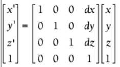 where dx = change in x, dy = change in y, and dz = change in z

Matrix4X1 translate3DByMultiply(Matrix start, float dx, float dy, float dz) {
    Matrix4X4 temp;
    Matrix4x1 result;

    // Zero out the matrix
    temp = createFixed4X4Matrix(0);

    // setup the 4X4 for multiplication
    temp.index[0][0] = 1;
    temp.index[1][1] = 1;
    temp.index[2][2] = 1;
    temp.index[3][3] = 1;

    // put in the translation amount
    temp.index[0][3] = dx;
    temp.index[1][3] = dy;
    temp.index[2][3] = dz;

    result = multiplyMatrixNxM(temp, start);
    return result;
}
Scaling
Matrix multiplication can also be used to scale objects in your game. Just like translation,if you scale each individual vertex, you end up scaling the whole object.
2D Scaling 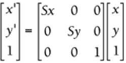 where Sx = scale factor in the x direction and Sy = scale factor in the y direction

Matrix3X1 scale2DByMultiplication(Matrix3X1 start, float dx, float dy) {
    Matrix3X3 temp;
    Matrix3X1 result;

    // Zero out the matrix
    temp = createFixed3X3Matrix(0);

    // setup the 3X3 for multiplication
    temp.index[0][0] = dx;
    temp.index[1][1] = dy;
    temp.index[2][2] = 1;

    result = multiplyMatrixNxM(temp, start);
    return result;
}
3D Scaling 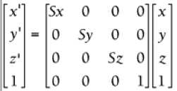 where Sx = scale factor in the x direction, Sy = scale factor in the y direction, and Sz = scale factor in the z direction

Matrix4X1 scale3DByMultiply(Matrix4X1 start, float dx, float dy, float dz) {
    Matrix4X4 temp;
    Matrix4X1 result;

    // Zero out the matrix to make sure nothing is left uninitialized
    temp = createFixed4X4Matrix(0);

    // setup the 3x3 for multiplication
    temp.index[0][0] = dx;
    temp.index[1][1] = dy;
    temp.index[2][2] = dz;
    temp.index[3][3] = 1;

    result = multiplyMatrixNxM(temp, start);
    return result;
}
Rotation
There are actually two different approaches to rotating objects. One method uses quaternions, but the math is complex. The other method is very similar to that of scaling and translating,because it uses a similar matrix equation.This second method is called Euler rotation
2D Rotation 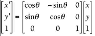 where q is the angle of rotation

Matrix3X1 rotate2D(Matrix3X1 start, float theta) {
    Matrix3X3 temp;
    Matrix3X1 result;
    // Zero out the matrix
    temp = createFixed3X3Matrix(0);
    // place the needed rotational values into the matrix
    temp.index[0][0] = cos(DegreesToRads(theta));
    temp.index[1][1] = cos(DegreesToRads(theta));
    temp.index[2][2] = 1;
    temp.index[0][1] = -1 * sin(DegreesToRads(theta));
    temp.index[1][0] = sin(DegreesToRads(theta));
    temp.index[2][2] = 1;
    result = multiplyMatrixNxM(temp, start);
    return result;
}
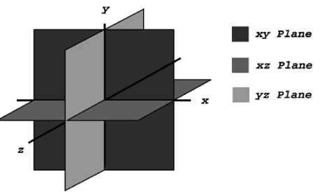
Notice that the xy plane is the same as the flat 2D plane you‘re used to working for the computer screen. Because there are three separate planes to rotate within, there are three separate rotation matrices for 3D
3D Rotation About the Z-Axis(Roll) 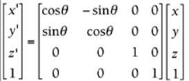 where q is the angle of rotation.

Matrix4X1 rotate3DZ(Matrix4X1 start, float theta) {
    Matrix4X4 temp;
    Matrix4X1 result;

    // Zero out the matrix
    temp = createFixed4X4Matrix(0);

    // put the needed rotation values into the matrix from theta
    temp.index[0][0] = cos(DegreesToRads(theta));
    temp.index[1][1] = cos(DegreesToRads(theta));
    temp.index[2][2] = 1;
    temp.index[3][3] = 1;

    temp.index[0][1] = -1 * sin(DegreesToRads(theta));
    temp.index[1][0] = sin(DegreesToRads(theta));

    result = multiplyMatrixNxM(temp, start);
    return result;
}
Concatenation
Concatenation is just a fancy name for combining transformation matrices into a single combo matrix.
This process can be used for any combination of translation,scaling, and rotation, not just the examples mentioned earlier. Any time you plan to perform more than one transformation within the same frame, you can save a lot of processor time by combining them.
It might take you more time up front when you‘re coding, but it will greatly enhance performance when the game is running


Matrix4X4 createRotationCombo(float thetax, float thetay, float thetaz) {
    Matrix4X4 X,Y,Z,temp,result;

    X = createFixed4X4Matrix(0.0f);
    Y = createFixed4X4Matrix(0.0f);
    Z = createFixed4X4Matrix(0.0f);
    temp = createFixed4X4Matrix(0.0f);
    result = createFixed4X4Matrix(0.0f);

    // place the needed X rotational values into the matrix
    X.index[0][0] = 1;
    X.index[1][1] = cos(DegreesToRads(thetax));
    X.index[2][2] = cos(DegreesToRads(thetax));
    X.index[3][3] = 1;

    X.index[2][1] = -1 * sin(DegreesToRads(thetax)));
    X.index[1][2] = sin(DegreesToRads(thetax));

    // place the needed Y-Axis rotational values into the matrix
    Y.index[0][0] = cos(DegreesToRads(thetay));
    Y.index[1][1] = 1;
    Y.index[2][2] = cos(DegreesToRads(thetay));
    Y.index[2][0] = -1 * sin(DegreesToRads(thetay));
    Y.index[0][2] = 1 * sin(DegreesToRads(thetay));

    // place the needed Z-axis rotational values into the matrix
    Z.index[0][0] = cos(DegreesToRads(thetaz));
    Z.index[1][1] = cos(DegreesToRads(thetaz));
    Z.index[2][2] = 1;
    Z.index[3][3] = 1;

    Z.index[0][1] = -1 * sin(DegreesToRads(thetaz));
    Z.index[1][0] = sin(DegreesToRads(thetaz));

    // Create the single Combo Matrix
    temp = multiply4X4Matrix(Y, X);
    result = multiply4X4Matrix(temp, Z);

    return result;
}

Matrix4X1 rotate3DWithCombo(Matrix4X4 combo, Matrix4X1 vertex) {
    Matrix4X1 temp;
    temp = multiplyMatrixNXM(combo, vertex);
    return temp;
}
2D Combo Matrix For every 2D combo matrix: 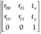 entries with an r store scaling and rotation information, and entries with at store overall translation information.
3D Combo Matrix 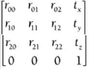 entries with an r store scaling and rotation information, and entries with at store overall translation information.
Conversion Between the OpenGL and DirectX Formats AB = BTAT for matrices A and B: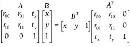
Visualization Experience
Self-Assessment Solutions
Chapter 7. Unit Convensions
The Metric System
Converting Units Between Systems
Computer Conversions
Self-Assessment Solutions
Chapter 8. Motion in One Dimension
Speed and Velocity
Any time an object is moving, it has some speed. Speed measures how fast an object is moving.If an object has speed, it also has a velocity, which is simply the vector version of speed.
Displacement with Constant Velocity displacement = velocity * time (D = v * t) for any constant velocity v.
If you chose to ignore direction, the same formula applies to the scalar equivalents: distance = speed * time for any constant speed.
Displacement Between Frames New_position = Old_position + Velocity * Time where Time is one frame (usually 1 / 30th of a second)
The framerate will most likely not stay constant at 30fps. Most developers calculate a "delta time" by subtracting the system clock‘s value at the last frame simulation from the value at this simulation and then use that as the time factor.
Average Velocity  for any displacement Dx and time interval t.
Acceleration
Acceleration 
Equations of Motion
Equation 1 vf = vi + at final velocity = initial velocity + acceleration * time
Equation 2 v = (vi + vf) / 2 average velocity = (inital velocity + final velocity ) / 2 for constant velocity only
Equation 3 Dx = 1/2(vi + vf)t displacement = 1/2(inital velocity + final velocity) * time
Equation 4 Dx = vi * t + 1/2*a*t2 displacement = inital velocity * time + 1/2 acceleration * time2
Equation 5 vf2 = vi2 + 2aΔx final velocity2 = initial velocity2 + 2 * acceleration * displacement
Visualization Experience
Self-Assessment Solutions
Chapter 9. Derivative Approach to Motion in One Dimension
Visualizing Velocity and Derivative
Average Velocity v = (f(b) - f(a)) / (b - a)
Instantaneous Velocity  at t = a for any function f(t) that gives position as a function of time.
Instantaneous Velocity v = f‘(t) for any position equation that‘s a function of time, f‘(t)
Average Acceleration a = (f(b) - f(a)) / (b - a)
Instantaneous Acceleration  for any function f(t) that gives velocity as a function of time.
Instantaneous Acceleration a = v‘(t) for any velocity equation that‘s a function of time, v(t)
Instantaneous Acceleration a = v‘(t) = y‘‘(t) for any velocity equation that‘s a function of time, v(t) and any position equation that‘s a function of time, y(t).
Visualizing Acceleration and Second Derivative
Self-Assessment Solutions
Chapter 10. Motion in Two and Three Dimensions
Using Vectors
2D Displacement Dr = rf - ri for position vectors ri(initial) and rf(final)

#include "3Dvector.h"

int main() {
    // Define our 2 vectors
    3Dvector inital(150, 0, 250);
    3Dvector final(400, 250, -300);
    // Calculate our solution
    3Dvector displacement = final - inital;

    return 0;
}
Let‘s look back at the definition of velocity in one dimension. Velocity is the rate of change of position. In two dimensions velocity is still displacement divided by time. The only difference is that now displacement is a 2D or 3D vector instead of a positive or negative number. This means that to calculate average velocity, you need to divide the vector displacement by the scalar time.
If the vector is in polar coordinates, simply divide the magnitude by time and keep the direction the same. If it‘s in Cartesian coordinates, divide each component by time. In either case , the definition is the same.
Average Velocity in 2D and 3D  for any displacement vector Dr and time interval t.

3Dvector averageVelocity(const 3Dvector &Pi, const 3Dvector &Pf, float intervals) {
    // Calculate the displacement between our start and finish
    3Dvector temp(Pf.x - Pf.y, Pf.y - Pi.y, Pf.z - Pi.z);
    // Divide our displacement by our number of intervals
    temp = temp * (1 / intervals);
    // Return our answer
    return temp;
}
Equations of Motion in 2D and 3D 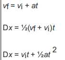 for vectors a, vf, vi, and Dx and scalar t.
These three equations are called parametric equations because the are functions of time. You‘ll find that they are used the most in game programming.

// purpose: calculate final velocity, given initial velocity, acceleration
// and time
// input: vi - initial velocity
//           a - acceleration
//           t -  time
// output: our final velocity
float eqOne_vf(float vi, float a, float t) {
    return vi + a * t;
}

// purpose: calculate change in distance, given final velocity, initial
// velocity, and time
// input: vf - final velocity
//           vi - initial velocity
//           t  - time
float eqTwo_x(float vf, float vi, float t) {
    return 0.5f * (vf - vi) / t;
}

// purpose: calculate change in distance, given initial velocity,
// acceleration, and time
// input: vi - initial velocity
//           t  - time
//            a - acceleration
// output: our change in distance
float eqThree_x(float vi, float t, float a) {
    return vi * t + 0.5f * a * t * t;
}

// purpose: calculate acceleration, given initial velocity,
// change in distance, and time
// input: vi - initial velocity
//            t - change in distance
//            a - acceleration
// output: our acceleration
float eqThree_a(float vi, float x, float a) {
    return (x - vi * t) * 2 / (t * t);
}
Projectiles
Any object that has been thrown, kicked, or shot and that is flying through the air is considered a projectile.
Vertical Components of a Projectile 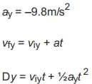
Horizontal Components of a Projectile
Visualization Experience
Self-Assessment Solutions
Chapter 11. Newton‘s Laws
Forces
Weight w = mg where m = mass and g = acceleration due to gravity (-9.8 m/s2 on Earth)
While most games won‘t need to differentiate between mass and weight, in extremely detailed games (or any simulation) such a distinction is needed.

// purpose: to calculate the weight of an object based on its mass
// input: mass - the mass of the object
//           grav  - the amount of constant acceleration due to gravity
// output: an array of 3 floats representing the vector of weight
float * calcWeight3D(float mass, float grav) {
    // This will hold the weight of the object until it returned
    // The value in [1] will be the only number changed, since gravity
    // is only applied along the Y axis
    float weight[3] = {0, 0, 0 };
    // Calculate the weight, it is assumed that grav is a negative number
    weight[1] = mass * grav;
    // Return our answer
    return weight;
}
Let‘s look a littile closer at mass and weight. The biggest difference between the two is that mass is a scalar quantity, and weight is a vector quantity.Even though we tend to use these two terms interchangeably in everyday language,in physics the are two very different
quantities. The units are often a dead giveaway as to which quantity you are working with.Mass often is measured in either grams or kilograms, whereas weight is measured in pounds or newtons.
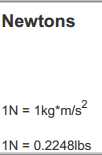
You might not be familiar with newtons, so let‘s define this new unit. If mass is measured in kilograms, when you multiply it by the acceleration due to gravity(g = -9.8m/s2) to calculate the object‘s weight on Earth, you end up with the unit of kg * m/s2. This unit is quite
awkward to say, so it has been named the Newton(written N) after Sir Isaac Newton. Unfortunately, you might be accustomed to approximating weights in pounds, so you might need to convert a weight from pounds to newtons. The conversion factor is 1N = 0.2248lbs.
Using Newton‘s Laws to Determine How Forces Affect an Object‘s Motion
Newton‘s First Law If Fnet = 0, there‘s no change in motion
Newton‘s Second Law Fnet = ma where m = mass and a = acceleration
Newton‘s Third Law For every force there is an equal and opposite force, or, when two objects come into contact, they exert equal and opposite forces upon each other
Self-Assessment Solutions
Chapter 12. Energy
Work and Kinetic Energy
In physics, work has a very precise definition. Work is equal to force times displacement
Work W = FDx where Dx = displacement and F = force in the directionfo displacement.
Joule(J) 1J = 1N*m

float calculateWork(float force, float friction, float displacement) {
    // calculate the difference of the forces
    float netForce = force - friction;
    // multiply by displacement
    float temp = displacement * netForce;
    return temp;
}

float caculateAngleWork(vector2D vect, float friction, float displacement) {
    float temp;
    // don‘t forget to convert to rads...
    temp = cos(DegreeToRads(vect.y));
    // calculate the horizontal force;
    float horizForce = vect.x * temp;
    float work = calculateWork(horizForce, friction, displacement);
    return work;
}

float calculateAngleWorkFromVector(vector2D initial, vector2D change) {
    vector2D force, displacement, displacementNormal, temp;
    float projectionLength, work;
    // change vectors from Polar to Cartesian
    force = polarToCartesian(initial);
    displacement = polarToCartesian(change);
    // Normalize the displacementNormal
    displacementNormal = normalizeVector(displacement);
    // the length of the project is the dot product of the
    // force against the displacement normal.
    projectionLength = dotProduct(force, displacementNormal);
    // Let‘s see what that length is
    cout << "Projection Length" << projectionLength << "\n";
    // multiply projection times normalized displacement Vector
    temp = scalarMultiply(projectionLength, displacementNormal);
    // Get back to Polar coordinates to calculate work. Don‘t forget
    // about radians
    temp = cartesianToPolar(temp);
    // Finally, our work is calculated
    work = temp.x * change.x;
    return work;
}

vector3D normalizeVector(vector3D vect) {
    float mag,square;
    vector3D temp;
    square = squareVector(vect);
    mag = sqrt(square);

    temp.x = vect.x/mag;
    temp.y = vect.y/mag;
    temp.z = vect.z/mag;
    return temp;
}

float dotProduct(vector3D a, vector3D b) {
    vector3D temp;
    float scalar;
    temp.x = a.x * b.x;
    temp.y = a.y * b.y;
    temp.z = a.z * b.z;
    scalar = sumVector(temp);
    return scalar;
}
Remember that work is a scalar quantity. so as soon as the force and displacement are in the same direction, you can ignore it and simply multiply the magnitudes
Kinetic energy is the amount of energy an object has because it is moving. Therefore, the faster it‘s moving, the more kinetic energy it has. In that respect, it‘s very similar to momentum, which is mass times velocity
The definition of kinetic energy is one-half of the mass times the speed squared, 1/2mv2
Kinetic Energy KE = 1/2mV2 where m = mass and v = speed.
Notice that the definition is based on speed rather than velocity.(Remember that speed is the scalar version of velocity, so it‘s the velocity minus its direction)

float calculateKineticEnergy(float mass, float speed) {
    float KE;
    KE = (mass/2)*(pow(speed,2));
    return KE;
}
Work-energy theorem,this theorem states that the net or total work done on an object is equal to the change in it‘s kinetic energy.
Wok-Energy Theorem W = DKE = KEf - KEi or FΔx = 1/2mvf2 - 1/2mvi2 where the force and displacement are in the same direction, and v is speed

float calculateWorkEnergy(float force, float mass, float displacement, float velocityInitial) {
    float work,vFinal;
    work = calculateWork(force, displacement);
    vFinal = work/((mass/2 - calculateKE(mass, velocityInitial));
    velocityFinal = sqrt(Final);
    return vFinal;
}
Gravitational Potential Energy GPE = mgy where m = mass, g = acceleration due to gravity, and y = height.
There are other types of potential energy, but they are relatively insignificant in terms of motion in a video game, so it‘s safe to ignore them. From this point forward we‘ll juse use PE to represent gravitational potential energy, because it‘s the only type we‘re concerned with

#define GRAVITY 9.81
float calculatePotentialEnergy(float mass, float height) {
    float PE;
    PE = mass * GRAVITY * height;
    return PE:
}
Potential Energy and the Conservation Law
Conservation of Mechanical Energy (Simplified) KEi + PEi = KEf + PEf or 1/2mvi2 + mgyi = 1/2mvf2 + mgyf
Conservation of Mechanical Energy (Modified) KEi + PEi = KEf + PEf + E0 or 1/2mvi2 + mgyi = 1/2mvf2 + mgyf + E0 where E0 represents other energy (heat/sound)
When you use this modified form, just make sure you extra term for heat and sound energy is relatively small compared to the other two forms fo energy. This is simple(and fast) cheat for modeling more realistic motion.
Self-Assessment Solutions
Chapter 13. Momentum and Collisions
Collision with a Stationary Object
Axis-Aligned Vector Reflection If the stationary boundary is vertical, vf = [-vix viy] and if the stationary boundary is horizontal, vf = [vix -viy] for incoming velocity vi = [vix viy]

vector2D axisAlignedCollision(vector2D vect, char b) {
    vector2D temp = vect;
    if (b == ‘v‘) {
        temp.x = temp.x *= -1;
    } else if (b == ‘h‘) {
        temp.y = temp.y *= -1;
    }

    return temp;
}
Non-Axis-Aligned Vector Reflection vf = 2 * P + vi where vi = the incoming velocity and P = the projection of -vi onto the normal of the boundary line

vector2D nonAxisAlignedCollision(vector2D a, vector2D b) {
    vector2D temp, temp2, temp3, length, reflection;
    float projection;
    temp = normalizeVector(a);
    // reverse the vector
    temp2 = scalarMultiply(-1, b);
    // find the projection length using the dot product
    projection = dotProduct(temp2, temp);
    length = scalarMultiply(projection, temp);
    // the reflection is going to be twice the length
    reflection = scalarMultiply(2, length);
    // sum them all together making sure the reflection is inverted
    temp3 = sumVectors(scalarMultiply(-1, reflection),temp2);

    return temp3;
}

vector3D nonAxisAlignColl(vector3D a, vector3D b, vector3D velocity) {
    vector3D temp, normal, velocityTemp, velocityFinal, length, reflection;
    velocityTemp = scalarMultiply(-1, velocity);
    float projection;
    temp = crossProduct(a, b);
    // get the surface normal
    normal = normalizeVector(temp);
    // calculate the projection
    projection = dotProduct(velocityTemp, normal);
    // Take the length of the projection against the normal
    length = scalarMultiply(projection, normal);
    // Lets obtain the final vector
    reflection = scalarMultiply(2, length);
    velocityFinal = sumVectors(reflection, velocity);
    return velocityFinal;
}
Momentum and Impulse Defined
The first step in the progress of modeling collision between two moving objects is to define a new quantity----momentum.Momentum(p) is defined as mass times velocity. This means that the more massive an object is, the more momentum it has.
That‘s why it‘s extremely difficult to bring a tractor-trailer to an abrupt stop. Likewise, a large velocity also results in a lot of momentum, so even if you‘re driving a little sports car, it‘s still difficult to stop at 100mph
Momentum p = mv where m= mass and v = velocity
Modeling Collisions
Visualization Experience
Self-Assessment Solutions
Chapter 14. Rotational Motion
Cicular Motion
Rotational Dynamics
Self-Assessment Solutions
Appendix B. Suggested Reading
Math
Dolciani, Mary P. et al.Algebra 2 and Trigonometry. Boston: Houghton Mifflin, 1992.
Finney, Ross L. et al.Calculus: Graphical, Numerical, Algebraic. Reading: Addison-Wesley, 1995.
Lecky-Thompson, Guy.Infinite Game Universe: Mathematical Techniques. Rockland: Charles River Media, 2001.
Leduc, Steven A.Linear Algebra. Lincoln: Cliffs Notes, 1996.
Stewart, James.Calculus. Pacific Grove: Brooks/Cole, 2002.
Strang, Gilbert.Introduction to Linear Algebra. Wellesley: Wellesly-Cambridge Press, 1993.
Thompson, Silvanus P. and Martin Gardner.Calculus Made Easy. New York: St. Martin‘s Press, 1998 (original copyright 1910).
Physics
Bourg, David M.Physics for Game Developers. Cambridge: O‘Reilly, 2002.
Gonick, Larry and Art Huffman.The Cartoon Guide to Physics. New York: HarperPerennial, 1990.
Huetinck, Linda.Physics. Lincoln: Cliffs Notes, 2001.
Serway, Raymond A. and Jerry S. Faughn.College Physics. Philadelphia: Saunders College Publishing, 2003.
3D Game Engineering
DeLoura, Mark, ed.Game Programming Gems. Rockland: Charles River Media, 2000.
DeLoura, Mark, ed.Game Programming Gems 2. Rockland: Charles River Media, 2001.
Dunn, Fletcher and Ian Parberry.3D Math Primer for Graphics & Game Development. Wordware, 2002.
Eberly, David H.3D Game Engine Design. San Francisco: Morgan Kaufmann Publishers, 2001.
Foley, J.D. and A. Van Dam.Fundamentals of Interactive Computer Graphics. Reading: Addison-Wesley, 1982.
LaMothe, Andre.Tricks of the Windows Game Programming Gurus. Indianapolis: Sams, 1999.
Lengyel, Eric.Mathematics for 3D Game Programming & Computer Graphics. Rockland: Charles River Media, 2001.
Watt, Alan and Fabio Policarpo.3D Games: Real-time Rendering and Software Technology. Reading: Addison-Wesley, 2001.
General Programming
Eckel, Bruce.Thinking in C++, Volume I: Introduction to Standard C++, Second Edition. Upper Saddle River: Prentice Hall, 2000.
Meyers, Scott.Effective C++: 50 Specific Ways to Improve Your Programs and Designs . Reading: Addison-Wesley, 2001.
Prata, Stephen.C++ Primer Plus , Third Edition. Indianapolis: Sams, 1998.
Beginning Math and Physics For Game Programmers
标签:example nis point fixed index gravity sim version run
原文地址:https://www.cnblogs.com/revoid/p/9728432.html