标签:data ret org dia package 预测 加载 pre single
注:在很长一段时间,MNIST数据集都是机器学习界很多分类算法的benchmark。初学深度学习,在这个数据集上训练一个有效的卷积神经网络就相当于学习编程的时候打印出一行“Hello World!”。下面基于与MNIST数据集非常类似的另一个数据集Fashion-MNIST数据集来构建一个卷积神经网络。
MNIST数据集在机器学习算法中被广泛使用,下面这句话能概况其重要性和地位:
In fact, MNIST is often the first dataset researchers try. "If it doesn‘t work on MNIST, it won‘t work at all", they said. "Well, if it does work on MNIST, it may still fail on others."
Fashion-MNIST数据集是由ZALANDO实验室制作,发表于2017年。在该数据集的介绍中,列出了MNIST数据集的不足之处:
- MNIST太容易了,卷积神经网络可以达到99.7%的正确率,传统的分类算法也能很轻易的达到97%的正确率;
- 被过度使用了;
- 不能很好的代表现代计算机视觉任务.
Fashion-MNIST数据集的规格(28×28像素的灰度图片,10个不同类型),数据量(训练集包括60000张图片,测试集包括10000张图片)都与MNIST保持一致。差别是,MNIST的数据是手写数字0-9,Fashion-MNIST的数据是不同类型的衣服和鞋的图片。
下面是该数据集中的标签:
| Label | Description |
|---|---|
| 0 | T-shirt/top |
| 1 | Trouser |
| 2 | Pullover |
| 3 | Dress |
| 4 | Coat |
| 5 | Sandal |
| 6 | Shirt |
| 7 | Sneaker |
| 8 | Bag |
| 9 | Ankle boot |
下面是一些例子:
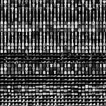
图0-1:Fashion-MNIST 中的图片示例
为了便于使用,TF收集了常用的数据集,制作成了一个独立的 Python package。可以通过以下方式安装:
- 更多关于该数据集的信息可参考:https://github.com/tensorflow/datasets
pip install -U tensorflow_datasets
下面导入了一些必要的package(包括前面安装的 tensorflow_datasets),并且输出了当前使用的 TensorFlow(TF) 的版本号。如果不是最新的TF,可以使用下面的命令安装最新的TF。
pip install tensorflow==2.0.0-alpha0 # 安装最新版的TF
 1 from __future__ import absolute_import, division, print_function
 2
 3
 4 # Import TensorFlow and TensorFlow Datasets
 5 import tensorflow as tf
 6 import tensorflow_datasets as tfds
 7
 8 # Helper libraries
 9 import math
10 import numpy as np
11 import matplotlib.pyplot as plt
12
13 # Improve progress bar display
14 import tqdm
15 import tqdm.auto
16 tqdm.tqdm = tqdm.auto.tqdm
17
18
19 print(tf.__version__) # 2.0.0-alpha0
20
21 # This will go away in the future.
22 # If this gives an error, you might be running TensorFlow 2 or above
23 # If so, the just comment out this line and run this cell again
24 # tf.enable_eager_execution()
准备就绪,就可以从 tensorflow_datasets 中导入Fashion-MNIST数据集了:
- 加载的过程中,会自动 shuffle 数据;
- 该数据集与MNIST数据集相同,train_dataset 中包含60000张图片用来做训练集,test_dataset 中包含10000张图片用来做测试集.
dataset, metadata = tfds.load(‘fashion_mnist‘, as_supervised=True, with_info=True)
train_dataset, test_dataset = dataset[‘train‘], dataset[‘test‘]
下面是所有衣服或鞋的名称,其顺序与其前面列出的该数据集的标签顺序相同:
class_names = [‘T-shirt/top‘, ‘Trouser‘, ‘Pullover‘, ‘Dress‘, ‘Coat‘,
               ‘Sandal‘,      ‘Shirt‘,   ‘Sneaker‘,  ‘Bag‘,   ‘Ankle boot‘]
可以利用 metadata 来查看数据集的信息:
- 下面会输出训练集和测试集中样本的个数
# metadata包含一些关于该数据集的元信息,包括数据集的description, url, version等信息
num_train_examples = metadata.splits[‘train‘].num_examples
num_test_examples = metadata.splits[‘test‘].num_examples
print("Number of training examples: {}".format(num_train_examples))
print("Number of test examples:     {}".format(num_test_examples))
原始数据中图片的每个像素由[0, 255]区间上的整数表示。为了更好的训练模型,需要将所有的值都标准化到区间[0, 1]。
- 经过测试,如果不做这一步,最终在测试集的准确率会下降大概8%。
1 def normalize(images, labels):
2     images = tf.cast(images, tf.float32)  # Casts a tensor to a new type
3     images /= 255
4     return images, labels
5
6 # The map function applies the normalize function to each element in the train
7 # and test datasets
8 train_dataset =  train_dataset.map(normalize)
9 test_dataset  =  test_dataset.map(normalize)
预处理后的数据同样可以表示一张图片,下面取出测试集中的一张图片并显示:
# Take a single image, and remove the color dimension by reshaping
for image, label in test_dataset.take(1):
    break
# print(image.shape, label.shape)
image = image.numpy().reshape((28,28))

# Plot the image - voila a piece of fashion clothing
plt.figure()
plt.imshow(image, cmap=plt.cm.binary)
plt.colorbar()
plt.grid(False)
plt.show()
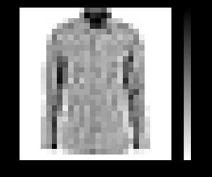
图1-1:标准化后的图片
取出训练集中前25张图片:
 1 plt.figure(figsize=(10,10))
 2 i = 0
 3 for (image, label) in train_dataset.take(25):
 4     image = image.numpy().reshape((28,28))
 5     plt.subplot(5,5,i+1)
 6     plt.xticks([])
 7     plt.yticks([])
 8     plt.grid(False)
 9     plt.imshow(image, cmap=plt.cm.binary)
10     plt.xlabel(class_names[label])
11     i += 1
12 plt.show()
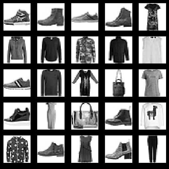
图1-2:训练集中前25张图片
准备好数据之后,就可以构建神经网络模型了。主要包括构建网络和编译两部分。
在构建网络时需要明确以下参数:
下面时构建网络的代码:
1 model = tf.keras.Sequential([
2     tf.keras.layers.Flatten(input_shape=(28, 28, 1)),
3     tf.keras.layers.Dense(128, activation=tf.nn.relu),
4     tf.keras.layers.Dense(10,  activation=tf.nn.softmax)
5 ])
该网络一共有3层(下面假设仅输入单个样本,即一张图片):
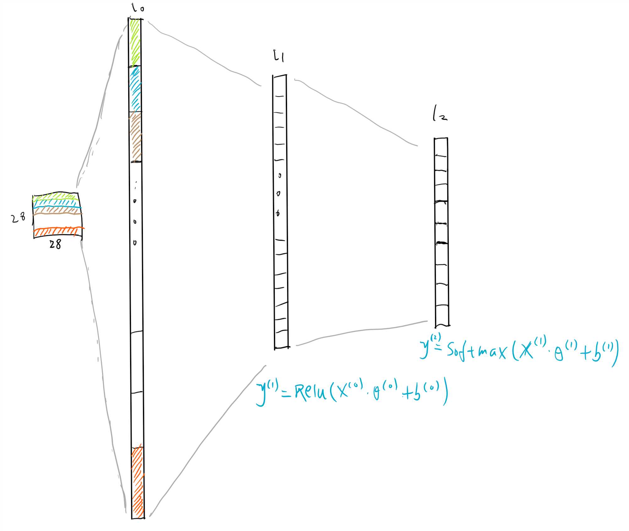
图1-3:网络的结构
上图中上角标表示层的编号,$\theta$表示各层的参数,$b$表示各层的偏执单元。
网络构建好之后,需要编译。在编译过程中需要确定以下几个参数:
损失函数与评估标准的异同:
下面是编译的代码:
model.compile(optimizer=‘adam‘,
              loss=‘sparse_categorical_crossentropy‘,
              metrics=[‘accuracy‘])
建立好模型之后,就可以训练模型了。因为是使用梯度下降来训练模型,因此除了训练集,还需要指定两个参数:
下面是训练模型的代码:
BATCH_SIZE = 32
train_dataset = train_dataset.repeat().shuffle(num_train_examples).batch(BATCH_SIZE)
test_dataset = test_dataset.batch(BATCH_SIZE)

model.fit(train_dataset, epochs=5, steps_per_epoch=math.ceil(num_train_examples/BATCH_SIZE))
下面是训练过程中的输出:
Epoch 1/5
1875/1875 [==============================] - 24s 13ms/step - loss: 0.2735 - accuracy: 0.8981
Epoch 2/5
1875/1875 [==============================] - 14s 8ms/step - loss: 0.2719 - accuracy: 0.8995
Epoch 3/5
1875/1875 [==============================] - 14s 8ms/step - loss: 0.2613 - accuracy: 0.9018
Epoch 4/5
1875/1875 [==============================] - 13s 7ms/step - loss: 0.2457 - accuracy: 0.9087
Epoch 5/5
1875/1875 [==============================] - 13s 7ms/step - loss: 0.2407 - accuracy: 0.9091
<tensorflow.python.keras.callbacks.History at 0x7fe5305bca58>
可以看到随着迭代次数的增加,损失函数的值在下降,分类的准确率在上升。最后该模型在训练集上的分类准确率为90.91%.
前面是在训练集中训练模型,训练的终止条件是人为设定的训练次数。训练停止后,模型在训练集上的分类准确率为91%。如果我们认为现在模型训练已经完成,最后一步就是在测试集上评价模型。测试集中包含的数据是模型之前从未见过新样本,如果在测试集上表现好,说明该模型有很好的泛化能力,学习到了这类数据的本质特征。
test_loss, test_accuracy = model.evaluate(test_dataset, steps=math.ceil(num_test_examples/32))
print(‘Accuracy on test dataset:‘, test_accuracy)
下面是输出:
313/313 [==============================] - 2s 6ms/step - loss: 0.3582 - accuracy: 0.8772
Accuracy on test dataset: 0.8772
因为测试集中每批次的大小也是32,因此需要重复10000/32=312.5次来完成整个测试集的测试。最终在测试集中分类准确率为88%,
下面从测试集取一个 batch 的样本(32个样本)进行预测,并将真实的label保存在test_labels中,最终得到第一个样本的预测分类与真实分类都是6.
for test_images, test_labels in test_dataset.take(1):
    test_images = test_images.numpy()
    test_labels = test_labels.numpy()
    predictions = model.predict(test_images)
np.argmax(predictions[0]), test_labels[0]  # (6, 6)
下面对部分结果进行可视化:
 1 def plot_image(i, predictions_array, true_labels, images):
 2     predictions_array, true_label, img = predictions_array[i], true_labels[i], images[i]
 3     plt.grid(False)
 4     plt.xticks([])
 5     plt.yticks([])
 6
 7     plt.imshow(img[...,0], cmap=plt.cm.binary)
 8
 9     predicted_label = np.argmax(predictions_array)
10     if predicted_label == true_label:
11         color = ‘blue‘
12     else:
13         color = ‘red‘
14
15     plt.xlabel("{} {:2.0f}% ({})".format(class_names[predicted_label],
16                                   100*np.max(predictions_array),
17                                   class_names[true_label]),
18                                   color=color)
19
20 def plot_value_array(i, predictions_array, true_label):
21     predictions_array, true_label = predictions_array[i], true_label[i]
22     plt.grid(False)
23     plt.xticks([])
24     plt.yticks([])
25     thisplot = plt.bar(range(10), predictions_array, color="#777777")
26     plt.ylim([0, 1])
27     predicted_label = np.argmax(predictions_array)
28
29     thisplot[predicted_label].set_color(‘red‘)
30     thisplot[true_label].set_color(‘blue‘)
31
32 # Plot the first X test images, their predicted label, and the true label
33 # Color correct predictions in blue, incorrect predictions in red
34 num_rows = 5
35 num_cols = 3
36 num_images = num_rows*num_cols
37 plt.figure(figsize=(2*2*num_cols, 2*num_rows))
38 for i in range(num_images):
39     plt.subplot(num_rows, 2*num_cols, 2*i+1)
40     plot_image(i, predictions, test_labels, test_images)
41     plt.subplot(num_rows, 2*num_cols, 2*i+2)
42     plot_value_array(i, predictions, test_labels)
结果如下:
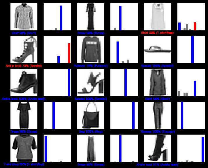
图1-4:部分结果的可视化
上图中,蓝色字体表示预测正确,蓝色柱状图表示正确的类;红色表示预测错误。
前面直接使用全连接层加上激活函数,已经取得了非常好分类效果:测试集的准确率为88%。实现卷积神经网络只需要改动网络的结构(1.4.1 构建网络)这一部分就可以了:
 1 model = tf.keras.Sequential([
 2     tf.keras.layers.Conv2D(32, (3,3), padding=‘same‘, activation=tf.nn.relu,
 3                            input_shape=(28, 28, 1)),
 4     tf.keras.layers.MaxPooling2D((2, 2), strides=2),
 5     tf.keras.layers.Conv2D(64, (3,3), padding=‘same‘, activation=tf.nn.relu),
 6     tf.keras.layers.MaxPooling2D((2, 2), strides=2),
 7     tf.keras.layers.Flatten(),
 8     tf.keras.layers.Dense(128, activation=tf.nn.relu),
 9     tf.keras.layers.Dense(10,  activation=tf.nn.softmax)
10 ])
此时,除了前面出现过的Flatten和Dense层,还有两种新的层类型:Conv2D和MaxPooling2D.
Conv2D表示二维卷积层(2D convolution layer),主要参数如下:
下面是卷积层处理的示意图:
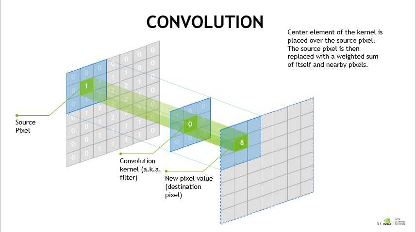
图2-1 卷积层过滤
上图左边是原图像,中间是过滤器,右边是卷积操作后得到的结果。
本文更多的是介绍 TF2.0 的实现方式,关于卷积层的更多知识点可以参考下面的链接:
- http://cs231n.stanford.edu/syllabus.html,Convolutional Neural Networks相关部分
- https://jhui.github.io/2017/03/16/CNN-Convolutional-neural-network/
MaxPooling2D表示2维最大池化层,用于对原图像进行下采用(down sampling),从而减小图片大小,降低训练难度。最大池化操作一般与卷积操作连在一起使用。主要参数如下:
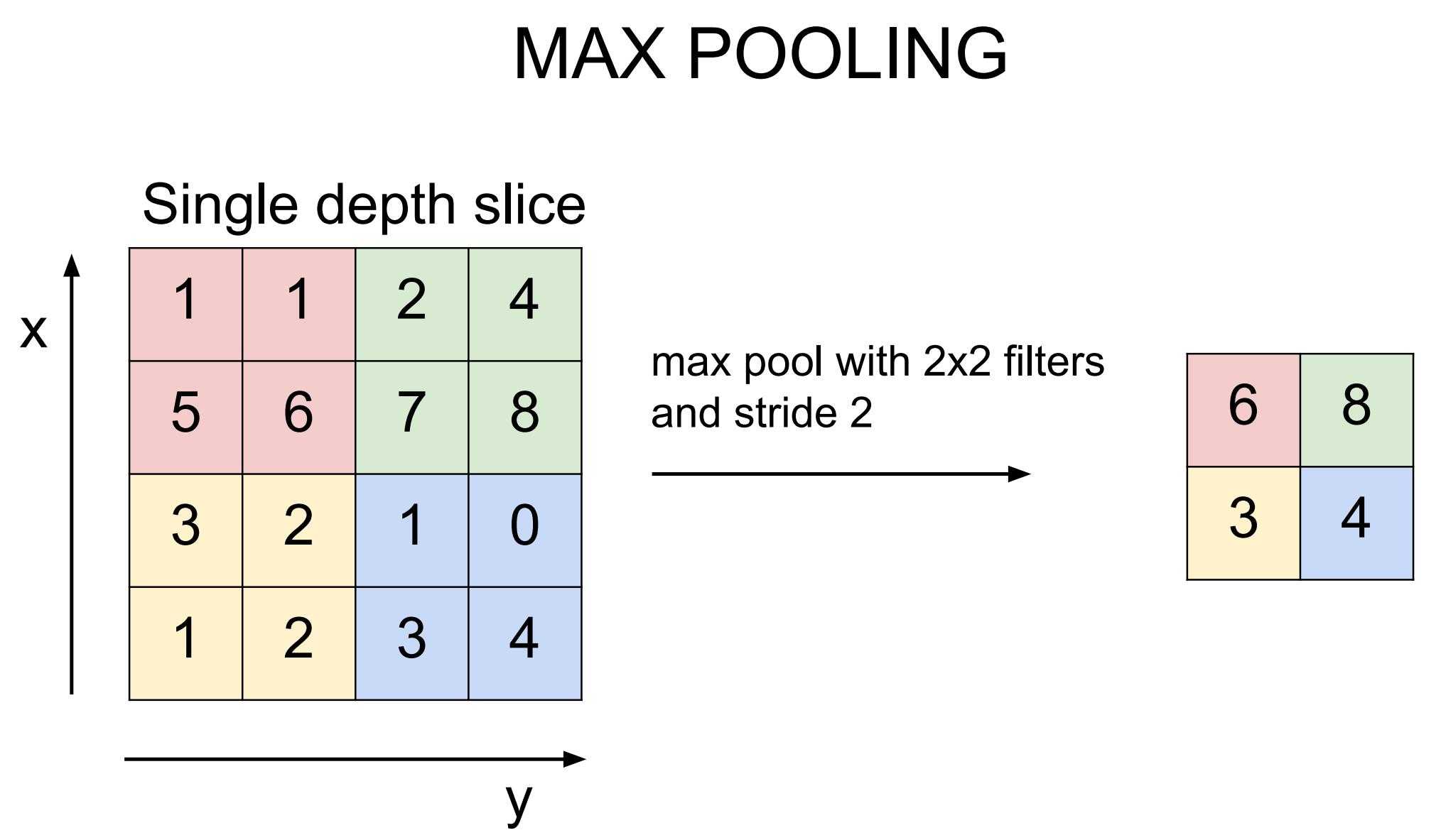
图2-2 使用(2, 2),步幅为2的窗口进行最大池化操作
最大池化就是只保留每个窗口中的最大值。如上图所示,按照(2, 2)的窗口大小和2的步幅,在左边(4, 4)的图像中只有4个窗口,每个窗口取最大值就可以得到右边的结果。
卷积神经网络之所以适合处理图片,一个最大的原因就是该算法具有位置不变性。例如进行图像识别时,不管所识别的物体位于图片的那个位置,都可以准确的识别。这种位置不变性就是卷积操作带来的,因为该操作使用一个小的窗口(kernal)地毯式的扫描了图片各个局部区域。
由卷积层和最大池化层构成的卷积神经网络将 Fashion-MNIST 测试集图片分类的正确率提高到了92%.
参考:https://keras.io/layers/about-keras-layers/
参考:https://keras.io/optimizers/
现在用的比较多的是RMSprop和Adam
https://github.com/zalandoresearch/fashion-mnist#why-we-made-fashion-mnist
https://arxiv.org/abs/1708.07747
https://medium.com/tensorflow/introducing-tensorflow-datasets-c7f01f7e19f3
https://towardsdatascience.com/a-comprehensive-guide-to-convolutional-neural-networks-the-eli5-way-3bd2b1164a53
https://datascience.stackexchange.com/questions/13663/neural-networks-loss-and-accuracy-correlation
https://keras.io/layers/convolutional/
https://keras.io/layers/pooling/
http://cs231n.stanford.edu/slides/2019/cs231n_2019_lecture05.pdf
https://blogs.nvidia.com/blog/2018/09/05/whats-the-difference-between-a-cnn-and-an-rnn/
https://github.com/OnlyBelter/examples/blob/master/courses/udacity_intro_to_tensorflow_for_deep_learning/l03c01_classifying_images_of_clothing.ipynb,代码
https://github.com/OnlyBelter/examples/blob/master/courses/udacity_intro_to_tensorflow_for_deep_learning/l04c01_image_classification_with_cnns.ipynb,代码
https://github.com/keras-team/keras-docs-zh,一些名词的翻译参考了该文档
Deep Learning with Python, by François Chollet, 2017.11
【深度学习与TensorFlow 2.0】卷积神经网络(CNN)
标签:data ret org dia package 预测 加载 pre single
原文地址:https://www.cnblogs.com/Belter/p/10662718.html