标签:直线 过程 str inline row 距离 学习 好的 nump
本文参考深入浅出--梯度下降法及其实现,对后面将公式转化为矩阵的形式加了些解释,便于大家理解。
梯度下降是用来求函数最小值点的一种方法,所谓梯度在一元函数中是指某一点的斜率,在多元函数中可表示为一个向量,可由偏导求得,此向量的指向是函数值上升最快的方向。公式表示为:
\[ \nabla J(\Theta) = \langle \frac{\overrightarrow{\partial J}}{\partial \theta_1}, \frac{\overrightarrow{\partial J}}{\partial \theta_2}, \frac{\overrightarrow{\partial J}}{\partial \theta_3} \rangle \]
比如
\[ \begin{aligned} J(\theta) &= \theta^2 \qquad \nabla J(\theta) = J'(\theta) = 2\theta\\ J(\theta) &= 2\theta_1+3\theta_2 \quad \nabla J(\theta) = \langle 2,3 \rangle \end{aligned} \]
由于梯度是函数值上升最快的方向,那么我们一直沿着梯度的反方向走,就能找到函数的局部最低点。
因此有梯度下降的递推公式:
\[ \Theta^1 = \Theta^0 - \alpha \nabla J(\Theta^0) \]
其中\(\alpha\)称为学习率,直观得讲就是每次沿着梯度反方向移动的距离,学习率过高可能会越过最低点,学习率过低又会使得学习速度偏慢。
为了更好的理解上面的公式
我们举例:
\[
\quad J(\theta) = \theta^2 \Longrightarrow \nabla J(\theta) = J'(\theta) = 2\theta
\]
则梯度下降的迭代过程有:
\[
\begin{aligned}
\theta^0 &= 1 \\theta^1 &= \theta^0 - \alpha \times J'(\theta^0) \\
&= 1-0.1 \times 2 \ &= 0.2 \\theta^2 &= \theta^1 - \alpha \times J'(\theta^1)\ &= 0.04\\theta^3 &= 0.008\\theta^4 &= 0.0016\\end{aligned}
\]
我们知道$J(\theta) = \theta^2 \(的极小值点在\)(0,0)\(处,而迭代四次后的结果\)(0.0016,0.00000256)$已相当接近。
再举一个二元函数的例子:
\[J(\Theta) = \theta_1^2 + \theta_2^2 \Longrightarrow \nabla J(\Theta) = \langle 2\theta_1 + 2\theta_2 \rangle\]
令\(\alpha = 0.1\), 以初始点\((1,3)\)用梯度下降法求函数最低点
\[
\begin{aligned}
\Theta^0 &= (1,3) \\Theta^1 &= \Theta^0 - \alpha \nabla J(\Theta^0)\ &= (1,3) - 0.1(2,6)\ &= (0.8,2.4)\\Theta^2 &= (0.8,2.4) - 0.1(1.6,4.8)\ &= (0.64,1.92) \\Theta^3 &= (0.512,1.536) \\end{aligned}
\]
值得注意的是,迭代的效率除了和步长(学习率)\(\alpha\)有关外,还与初始值的选取有关。
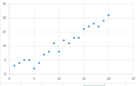
利用梯度下降法拟合出一条直线使得平均方差最小。
假设拟合后的直线为:
\[h_\Theta(x) = \theta_0 + \theta_1 \times x \]
其中\(\Theta = (\theta_0, \theta_1)\)
把平均方差作为代价函数
\[J(\Theta) = \frac{1}{2m}\sum_{i=1}^m \left\lbrace h_\Theta(x_i) - y_i \right\rbrace ^2\]
\[ \begin{aligned} &\nabla J(\Theta) = \langle \frac{\delta J}{\delta \theta_0}, \frac{\delta J}{\delta\theta_1} \rangle \&\frac{\delta J}{\delta \theta_0} = \frac{1}{m} \sum_{i=1}^m \left\lbrace h_\Theta(x_i) - y_i \right\rbrace\&\frac{\delta J}{\delta \theta_1} = \frac{1}{m} \sum_{i=1}^m \left\lbrace h_\Theta(x_i) - y_i \right\rbrace x_i\\end{aligned} \]
为了便于利用python的矩阵运算,我们可以将公式稍微变形
\[
\begin{aligned}
h_\Theta(x_i) &= \theta_0 \times 1 + \theta_1 \times x_i \ &=
\begin{bmatrix}
1 & x_0\ 1 & x_1\ \vdots & \vdots\ 1 & x_{19}\ \end{bmatrix}
\times
\begin{bmatrix}
\theta_0\ \theta_1
\end{bmatrix}
\end{aligned}
\]
\(i\)的范围是\([1,20]\),因此最后得到
\[
h_\Theta(x_i)=
\begin{bmatrix}
h_0\h_1\\vdots\h_{19}
\end{bmatrix}
\]
\[ 误差diff = \begin{bmatrix} h_0\h_1\\vdots\h_{19} \end{bmatrix}- \begin{bmatrix} y_0\y_1\\vdots\y_{19} \end{bmatrix} \]
\[ 方差和 \sum_{i=1}^m \left\lbrace h_\Theta(x_i) - y_i \right\rbrace ^2=diff^T \times diff \]
将公式变为矩阵向量相乘的形式后你应当更容易理解下面的python代码
import numpy as np

# Size of the points dataset.
m = 20

# Points x-coordinate and dummy value (x0, x1).
X0 = np.ones((m, 1))
X1 = np.arange(1, m+1).reshape(m, 1)
X = np.hstack((X0, X1))

# Points y-coordinate
y = np.array([
    3, 4, 5, 5, 2, 4, 7, 8, 11, 8, 12,
    11, 13, 13, 16, 17, 18, 17, 19, 21
]).reshape(m, 1)

# The Learning Rate alpha.
alpha = 0.01

def error_function(theta, X, y):
    '''Error function J definition.'''
    diff = np.dot(X, theta) - y
    return (1./(2*m)) * np.dot(np.transpose(diff), diff)

def gradient_function(theta, X, y):
    '''Gradient of the function J definition.'''
    diff = np.dot(X, theta) - y
    return (1./m) * np.dot(np.transpose(X), diff)

def gradient_descent(X, y, alpha):
    '''Perform gradient descent.'''
    theta = np.array([1, 1]).reshape(2, 1)
    gradient = gradient_function(theta, X, y)
    while not np.all(np.absolute(gradient) <= 1e-5):
        theta = theta - alpha * gradient
        gradient = gradient_function(theta, X, y)
    return theta

optimal = gradient_descent(X, y, alpha)
print('optimal:', optimal)
print('error function:', error_function(optimal, X, y)[0,0])标签:直线 过程 str inline row 距离 学习 好的 nump
原文地址:https://www.cnblogs.com/lepeCoder/p/10989348.html