《统计学习方法》第六章，逻辑斯蒂回归

  1 import numpy as np
  2 import matplotlib.pyplot as plt
  3 from mpl_toolkits.mplot3d import Axes3D
  4 from mpl_toolkits.mplot3d.art3d import Poly3DCollection
  5 from matplotlib.patches import Rectangle
  6 
  7 dataSize = 10000
  8 trainRatio = 0.3
  9 ita = 0.03
 10 epsilon = 0.01
 11 defaultTurn = 500
 12 colors = [[0.5,0.25,0],[1,0,0],[0,0.5,0],[0,0,1],[1,0.5,0]]                         # 棕红绿蓝橙
 13 trans = 0.5
 14 
 15 def sigmoid(x):
 16     return 1.0 / (1 + np.exp(-x))
 17 
 18 def function(x, para):                                                               # 回归函数
 19     return sigmoid(np.sum(x * para[0]) + para[1])
 20 
 21 def judge(x, para):                                                                 # 分类函数，由乘加部分和阈值部分组成
 22     return int(function(x, para) > 0.5)
 23 
 24 def dataSplit(x, y, part):    
 25     return x[:part], y[:part],x[part:],y[part:]
 26 
 27 def createData(dim, count = dataSize):                                              # 创建数据集
 28     np.random.seed(103)       
 29     X = np.random.rand(count, dim)
 30     Y = ((3 - 2 * dim)*X[:,0] + 2 * np.sum(X[:,1:], 1) > 0.5).astype(int)           # 只考虑 {0，1} 的二分类         
 31     class1Count = 0
 32     for i in range(count):
 33         class1Count += (Y[i] + 1)>>1   
 34     print("dim = %d, dataSize = %d, class 1 ratio -> %4f"%(dim, count, class1Count / count))
 35     return X, Y
 36 
 37 def stochasticGradientDescent(dataX, dataY, turn = defaultTurn):    
 38     count, dim = np.shape(dataX)
 39     xE = np.concatenate((dataX, np.ones(count)[:,np.newaxis]), axis = 1)    
 40     w = np.ones(dim + 1)    
 41     
 42     for t in range(turn):        
 43         y = sigmoid(np.dot(xE, w).T)
 44         error = dataY - y
 45         w += ita * np.dot(error, xE)
 46         if np.sum(error * error) < count * epsilon:
 47             break    
 48     return (w[:-1], w[-1])
 49 
 50 def test(dim):                                                
 51     allX, allY = createData(dim)
 52     trainX, trainY, testX, testY = dataSplit(allX, allY, int(dataSize * trainRatio))    # 分离训练集 
 53     
 54     para = stochasticGradientDescent(testX, testY)  # 训练   
 55     
 56     myResult = [ judge(x, para) for x in testX]                                     # 测试结果
 57     errorRatio = np.sum((np.array(myResult) - testY)**2) / (dataSize * (1 - trainRatio))
 58     print("dim = %d, errorRatio = %4f\n"%(dim, errorRatio))
 59     
 60     if dim >= 4:                                                                    # 4维以上不画图，只输出测试错误率
 61         return
 62     errorPX = []                                                                    # 测试数据集分为错误类，1 类和 0 类
 63     errorPY = []
 64     class1 = []
 65     class0 = []
 66     for i in range(len(testX)):
 67         if myResult[i] != testY[i]:
 68             errorPX.append(testX[i])
 69             errorPY.append(testY[i])
 70         elif myResult[i] == 1:
 71             class1.append(testX[i])
 72         else:
 73             class0.append(testX[i])
 74     errorPX = np.array(errorPX)
 75     errorPY = np.array(errorPY)
 76     class1 = np.array(class1)
 77     class0 = np.array(class0)
 78 
 79     fig = plt.figure(figsize=(10, 8))                  
 80     
 81     if dim == 1:
 82         plt.xlim(0.0,1.0)
 83         plt.ylim(-0.25,1.25)
 84         plt.plot([0.5, 0.5], [-0.5, 1.25], color = colors[0],label = "realBoundary")               
 85         plt.plot([0, 1], [ function(i, para) for i in [0,1] ],color = colors[4], label = "myF")
 86         plt.scatter(class1, np.ones(len(class1)), color = colors[1], s = 2,label = "class1Data")               
 87         plt.scatter(class0, np.zeros(len(class0)), color = colors[2], s = 2,label = "class0Data")               
 88         if len(errorPX) != 0:
 89             plt.scatter(errorPX, errorPY,color = colors[3], s = 16,label = "errorData")       
 90         plt.text(0.21, 1.12, "realBoundary: 2x = 1\nmyF(x) = " + str(round(para[0][0],2)) + " x + " + str(round(para[1],2)) + "\n errorRatio = " + str(round(errorRatio,4)), 91             size=15, ha="center", va="center", bbox=dict(boxstyle="round", ec=(1., 0.5, 0.5), fc=(1., 1., 1.)))
 92         R = [Rectangle((0,0),0,0, color = colors[k]) for k in range(5)]
 93         plt.legend(R, ["realBoundary", "class1Data", "class0Data", "errorData", "myF"], loc=[0.81, 0.2], ncol=1, numpoints=1, framealpha = 1)       
 94    
 95     if dim == 2:       
 96         plt.xlim(0.0,1.0)
 97         plt.ylim(0.0,1.0)
 98         plt.plot([0,1], [0.25,0.75], color = colors[0],label = "realBoundary")       
 99         xx = np.arange(0, 1 + 0.1, 0.1)               
100         X,Y = np.meshgrid(xx, xx)
101         contour = plt.contour(X, Y, [ [ function((X[i,j],Y[i,j]), para) for j in range(11)] for i in range(11) ])
102         plt.clabel(contour, fontsize = 10,colors=‘k‘)
103         plt.scatter(class1[:,0], class1[:,1], color = colors[1], s = 2,label = "class1Data")       
104         plt.scatter(class0[:,0], class0[:,1], color = colors[2], s = 2,label = "class0Data")       
105         if len(errorPX) != 0:
106             plt.scatter(errorPX[:,0], errorPX[:,1], color = colors[3], s = 8,label = "errorData")       
107         plt.text(0.71, 0.92, "realBoundary: -x + 2y = 1/2\nmyF(x,y) = " + str(round(para[0][0],2)) + " x + " + str(round(para[0][1],2)) + " y + " + str(round(para[1],2)) + "\n errorRatio = " + str(round(errorRatio,4)), 108             size = 15, ha="center", va="center", bbox=dict(boxstyle="round", ec=(1., 0.5, 0.5), fc=(1., 1., 1.)))
109         R = [Rectangle((0,0),0,0, color = colors[k]) for k in range(4)]
110         plt.legend(R, ["realBoundary", "class1Data", "class0Data", "errorData"], loc=[0.81, 0.2], ncol=1, numpoints=1, framealpha = 1)    
111 
112     if dim == 3:       
113         ax = Axes3D(fig)
114         ax.set_xlim3d(0.0, 1.0)
115         ax.set_ylim3d(0.0, 1.0)
116         ax.set_zlim3d(0.0, 1.0)
117         ax.set_xlabel(‘X‘, fontdict={‘size‘: 15, ‘color‘: ‘k‘})
118         ax.set_ylabel(‘Y‘, fontdict={‘size‘: 15, ‘color‘: ‘k‘})
119         ax.set_zlabel(‘W‘, fontdict={‘size‘: 15, ‘color‘: ‘k‘})
120         v = [(0, 0, 0.25), (0, 0.25, 0), (0.5, 1, 0), (1, 1, 0.75), (1, 0.75, 1), (0.5, 0, 1)]
121         f = [[0,1,2,3,4,5]]
122         poly3d = [[v[i] for i in j] for j in f]
123         ax.add_collection3d(Poly3DCollection(poly3d, edgecolor = ‘k‘, facecolors = colors[0]+[trans], linewidths=1))       
124         ax.scatter(class1[:,0], class1[:,1],class1[:,2], color = colors[1], s = 2, label = "class1")                      
125         ax.scatter(class0[:,0], class0[:,1],class0[:,2], color = colors[2], s = 2, label = "class0")                      
126         if len(errorPX) != 0:
127             ax.scatter(errorPX[:,0], errorPX[:,1],errorPX[:,2], color = colors[3], s = 8, label = "errorData")               
128         ax.text3D(0.74, 0.95, 1.15, "realBoundary: -3x + 2y +2z = 1/2\nmyF(x,y,z) = " + str(round(para[0][0],2)) + " x + " + 129             str(round(para[0][1],2)) + " y + " + str(round(para[0][2],2)) + " z + " + str(round(para[1],2)) + "\n errorRatio = " + str(round(errorRatio,4)), 130             size = 12, ha="center", va="center", bbox=dict(boxstyle="round", ec=(1, 0.5, 0.5), fc=(1, 1, 1)))
131         R = [Rectangle((0,0),0,0, color = colors[k]) for k in range(4)]
132         plt.legend(R, ["realBoundary", "class1Data", "class0Data", "errorData"], loc=[0.83, 0.1], ncol=1, numpoints=1, framealpha = 1)
133        
134     fig.savefig("R:\\dim" + str(dim) + ".png")
135     plt.close() 
136 
137 if __name__==‘__main__‘:
138     test(1)        
139     test(2)        
140     test(3)           
141     test(4)
142     test(5)   

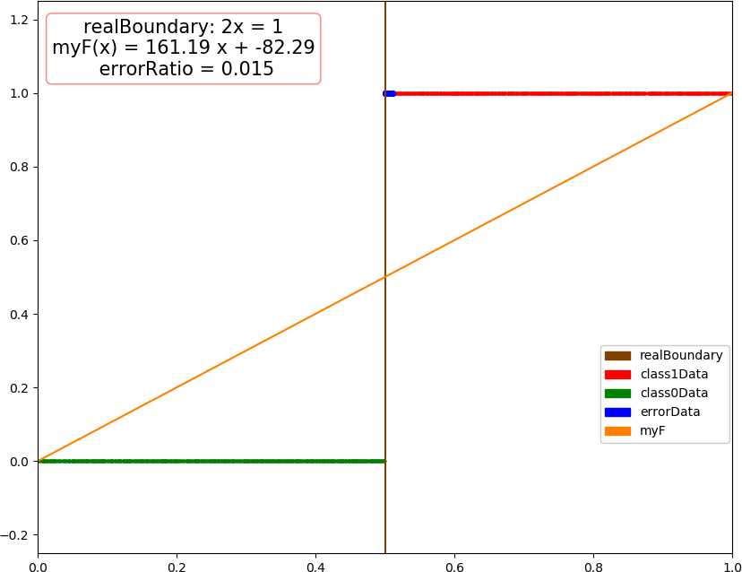
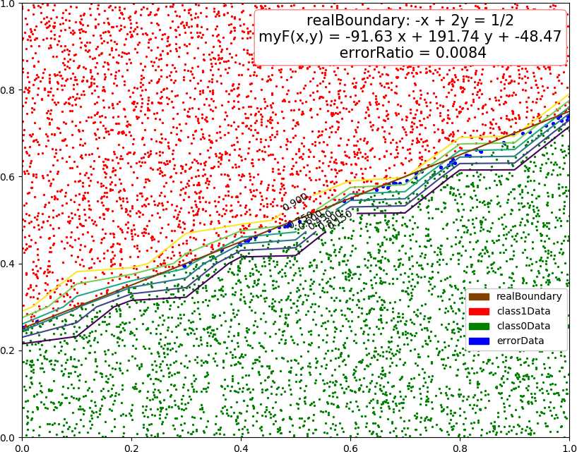
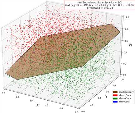
dim = 1, dataSize = 10000, class 1 ratio -> 0.509000
dim = 1, errorRatio = 0.015000

dim = 2, dataSize = 10000, class 1 ratio -> 0.496000
dim = 2, errorRatio = 0.008429

dim = 3, dataSize = 10000, class 1 ratio -> 0.498200
dim = 3, errorRatio = 0.012429

dim = 4, dataSize = 10000, class 1 ratio -> 0.496900
dim = 4, errorRatio = 0.012857

dim = 5, dataSize = 10000, class 1 ratio -> 0.500000
dim = 5, errorRatio = 0.012143