标签:RoCE tle 更新 add txt 作用 mod 函数 二维
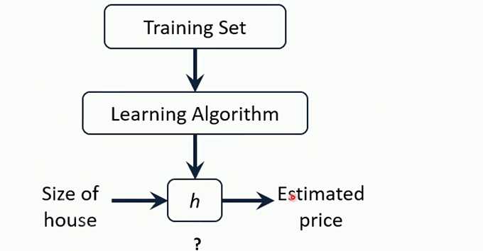
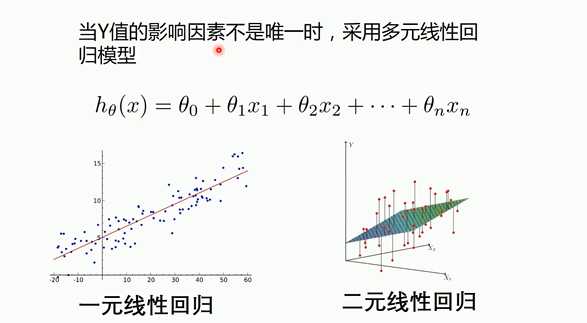
线性回归
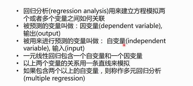
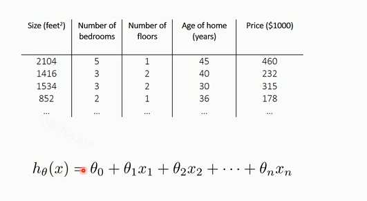
对于多元线性回归和一元线性回归推导理论是一致的,只不过参数是多个参数而已
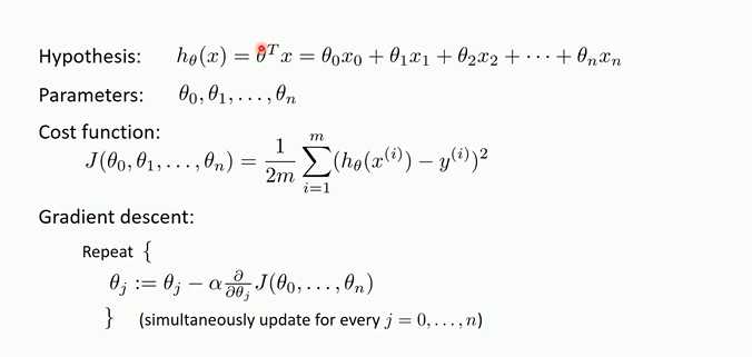
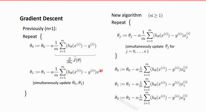
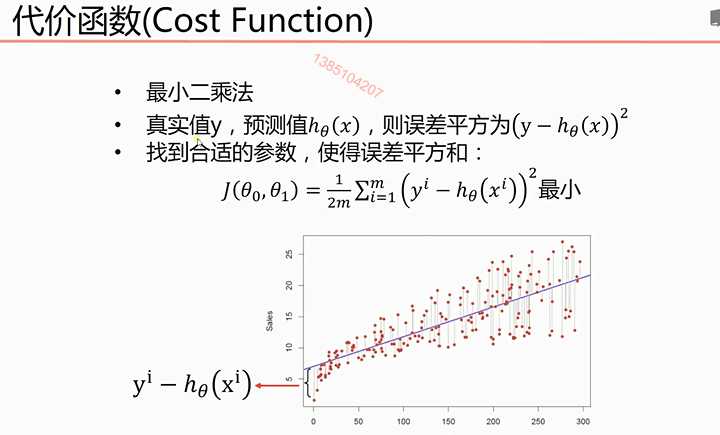
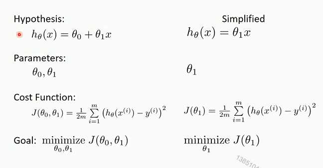
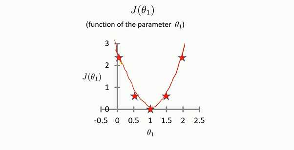
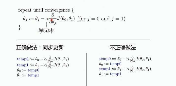
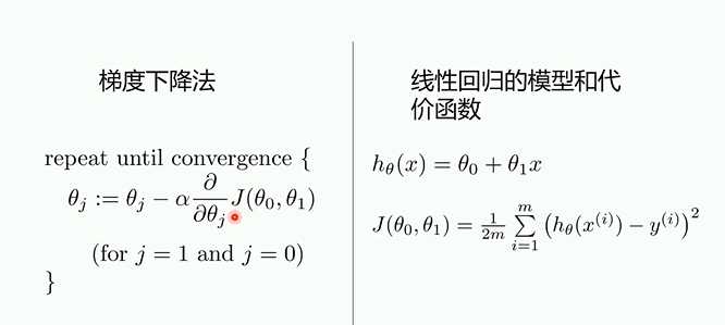
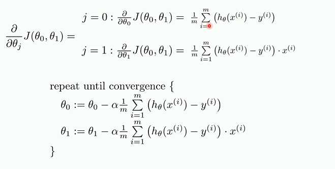
梯度下降
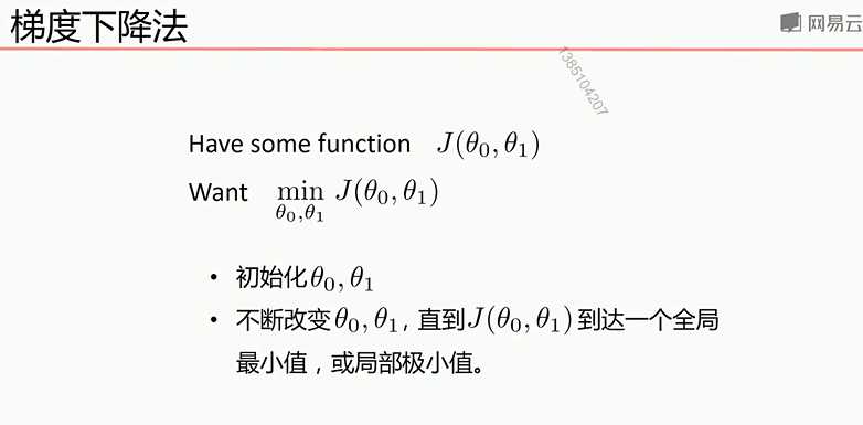
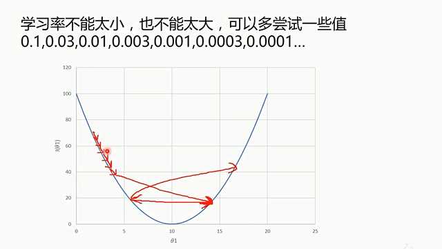
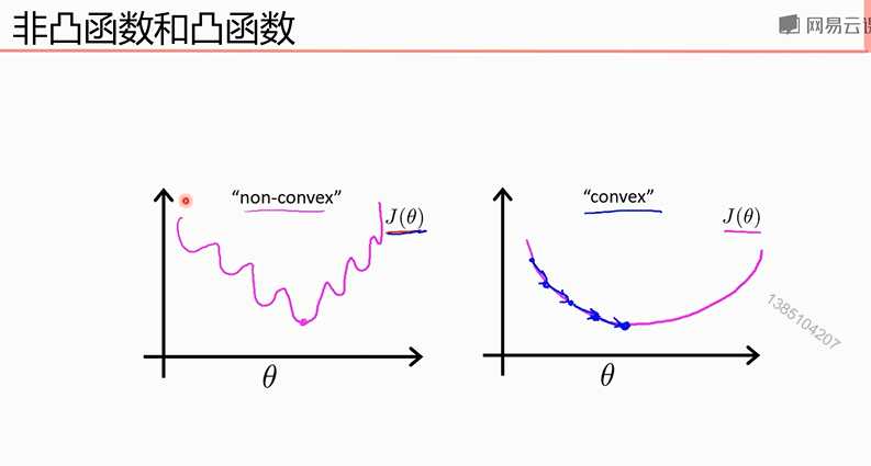
凸函数使用局部下降法一定可以到全部最小值,所以不存在局部最小值才可以
下面两个demo是一元函数的拟合
1使用梯度下降法的数学公式进行的机器学习代码
 1 import numpy as np
 2 from matplotlib import  pyplot as plt
 3 #读取数据
 4 data = np.genfromtxt(‘data.csv‘,delimiter=‘,‘)
 5 x_data = data[:, 0]
 6 y_data = data[:, 1]
 7 #plt.scatter(x_data, y_data)
 8 #plt.show()
 9 lr = 0.0001
10 k = 0
11 b = 0
12 epochs = 500
13 def compute_loss(x_data, y_data, b, k):#计算损失函数
14     m = float(len(x_data))
15     sum = 0
16     for i in range(0, len(x_data)):
17         sum += (y_data[i] - (k*x_data[i] + b))**2
18     return sum/(2*m)
19 def gradient(x_data, y_data, k, b, lr, epochs):#进行梯度下降
20     m = float(len(x_data))
21
22     for i in range(0,epochs):
23         k_gradient = 0
24         b_gradiet = 0
25         for j in range(0,len(x_data)):
26             k_gradient += (1/m)*((x_data[j] * k + b) - y_data[j])
27             b_gradiet += (1/m)*((x_data[j] * k + b) - y_data[j]) * x_data[j]
28         k -= lr * k_gradient
29         b -= lr * b_gradiet
30
31
32         if i % 50 == 0:
33             print(i)
34             plt.plot(x_data, y_data, ‘b.‘)
35             plt.plot(x_data, k*x_data + b, ‘r‘)
36             plt.show()
37
38     return k, b
39
40 k,b = gradient(x_data, y_data, 0, 0, lr, epochs)
41 plt.plot(x_data, k * x_data + b, ‘r‘)
42 plt.plot(x_data, y_data, ‘b.‘)
43 print(‘loss =:‘,compute_loss(x_data, y_data, b, k),‘b =:‘,b,‘k =:‘,k)
44 plt.show()
2 使用Python的sklearn库
 1 import numpy as np
 2 from matplotlib import  pyplot as plt
 3 from sklearn.linear_model import LinearRegression
 4 #读取数据
 5 data = np.genfromtxt(‘data.csv‘,delimiter=‘,‘)
 6 x_data = data[:, 0]
 7 y_data = data[:, 1]
 8 plt.scatter(x_data, y_data)
 9 plt.show()
10 x_data = data[:, 0, np.newaxis]#使一位数据编程二维数据
11 y_data = data[:, 1, np.newaxis]
12 model =LinearRegression()
13 model.fit(x_data, y_data)#传进的参数必须是二维的
14 plt.plot(x_data, y_data, ‘b.‘)
15 plt.plot(x_data, model.predict(x_data), ‘r‘)#画出预测的线条
16 plt.show()
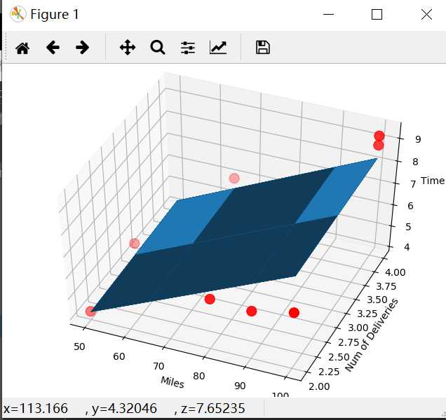
3使用梯度下降法完成多元线性回归(以二元为例)
 1 import numpy as np
 2 from numpy import genfromtxt
 3 import matplotlib.pyplot as plt
 4 from mpl_toolkits.mplot3d import Axes3D #用来画3D图的包
 5 # 读入数据
 6 data = genfromtxt(r"Delivery.csv",delimiter=‘,‘)
 7 print(data)
 8 # 切分数据
 9 x_data = data[:,:-1]
10 y_data = data[:,-1]
11 print(x_data)
12 print(y_data)
13 # 学习率learning rate
14 lr = 0.0001
15 # 参数
16 theta0 = 0
17 theta1 = 0
18 theta2 = 0
19 # 最大迭代次数
20 epochs = 1000
21
22 # 最小二乘法
23 def compute_error(theta0, theta1, theta2, x_data, y_data):
24     totalError = 0
25     for i in range(0, len(x_data)):
26         totalError += (y_data[i] - (theta1 * x_data[i,0] + theta2*x_data[i,1] + theta0)) ** 2
27     return totalError / float(len(x_data))
28
29 def gradient_descent_runner(x_data, y_data, theta0, theta1, theta2, lr, epochs):
30     # 计算总数据量
31     m = float(len(x_data))
32     # 循环epochs次
33     for i in range(epochs):
34         theta0_grad = 0
35         theta1_grad = 0
36         theta2_grad = 0
37         # 计算梯度的总和再求平均
38         for j in range(0, len(x_data)):
39             theta0_grad += (1/m) * ((theta1 * x_data[j,0] + theta2*x_data[j,1] + theta0) - y_data[j])
40             theta1_grad += (1/m) * x_data[j,0] * ((theta1 * x_data[j,0] + theta2*x_data[j,1] + theta0) - y_data[j])
41             theta2_grad += (1/m) * x_data[j,1] * ((theta1 * x_data[j,0] + theta2*x_data[j,1] + theta0) - y_data[j])
42         # 更新b和k
43         theta0 = theta0 - (lr*theta0_grad)
44         theta1 = theta1 - (lr*theta1_grad)
45         theta2 = theta2 - (lr*theta2_grad)
46     return theta0, theta1, theta2
47 print("Starting theta0 = {0}, theta1 = {1}, theta2 = {2}, error = {3}".
48       format(theta0, theta1, theta2, compute_error(theta0, theta1, theta2, x_data, y_data)))
49 print("Running...")
50 theta0, theta1, theta2 = gradient_descent_runner(x_data, y_data, theta0, theta1, theta2, lr, epochs)
51 print("After {0} iterations theta0 = {1}, theta1 = {2}, theta2 = {3}, error = {4}".
52       format(epochs, theta0, theta1, theta2, compute_error(theta0, theta1, theta2, x_data, y_data)))
53 ax = Axes3D(plt.figure())#和下面的代码功能一样
54 #ax = plt.figure().add_subplot(111, projection=‘3d‘)#plt.figure().add_subplot和plt.subplot的作用是一致的
55 ax.scatter(x_data[:, 0], x_data[:, 1], y_data, c=‘r‘, marker=‘o‘, s=100)  # 点为红色三角形
56 x0 = x_data[:, 0]
57 x1 = x_data[:, 1]
58 # 生成网格矩阵
59 x0, x1 = np.meshgrid(x0, x1)#生成一个网格矩阵,矩阵的每个点的第一个轴的取值来自于x0范围内,第二个坐标轴的取值来自于x1范围内
60 z = theta0 + x0 * theta1 + x1 * theta2
61 # 画3D图
62 ax.plot_surface(x0, x1, z)
63 # 设置坐标轴
64 ax.set_xlabel(‘Miles‘)
65 ax.set_ylabel(‘Num of Deliveries‘)
66 ax.set_zlabel(‘Time‘)
67
68 # 显示图像
69 plt.show()
4:使用Python的sklearn库完成多元线性回归
import numpy as np
from numpy import genfromtxt
from sklearn import linear_model
import matplotlib.pyplot as plt
from mpl_toolkits.mplot3d import Axes3D
# 读入数据
data = genfromtxt(r"Delivery.csv",delimiter=‘,‘)
print(data)
# 切分数据
x_data = data[:,:-1]
y_data = data[:,-1]
print(x_data)
print(y_data)
# 创建模型
model = linear_model.LinearRegression()
model.fit(x_data, y_data)
# 系数
print("coefficients:",model.coef_)

# 截距
print("intercept:",model.intercept_)

# 测试
x_test = [[102,4]]
predict = model.predict(x_test)
print("predict:",predict)
ax = plt.figure().add_subplot(111, projection=‘3d‘)
ax.scatter(x_data[:, 0], x_data[:, 1], y_data, c=‘r‘, marker=‘o‘, s=100)  # 点为红色三角形
x0 = x_data[:, 0]
x1 = x_data[:, 1]
# 生成网格矩阵
x0, x1 = np.meshgrid(x0, x1)
z = model.intercept_ + x0*model.coef_[0] + x1*model.coef_[1]
# 画3D图
ax.plot_surface(x0, x1, z)#参数是二维的,而model.prodict(x_data)是一维的。
# 设置坐标轴
ax.set_xlabel(‘Miles‘)
ax.set_ylabel(‘Num of Deliveries‘)
ax.set_zlabel(‘Time‘)

# 显示图像
plt.show()
5 多项式回归拟合
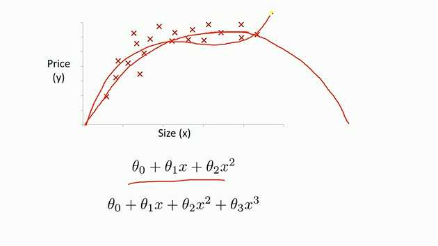

 1 import numpy as np
 2 import matplotlib.pyplot as plt
 3 from sklearn.preprocessing import PolynomialFeatures#多项式
 4 from sklearn.linear_model import LinearRegression
 5
 6 # 载入数据
 7 data = np.genfromtxt("job.csv", delimiter=",")
 8 x_data = data[1:,1]
 9 y_data = data[1:,2]
10 plt.scatter(x_data,y_data)
11 plt.show()
12 x_data
13 x_data = x_data[:,np.newaxis]
14 y_data = y_data[:,np.newaxis]
15 x_data
16 # 创建并拟合模型
17 model = LinearRegression()
18 model.fit(x_data, y_data)
19 # 画图
20 plt.plot(x_data, y_data, ‘b.‘)
21 plt.plot(x_data, model.predict(x_data), ‘r‘)
22 plt.show()
23 # 定义多项式回归,degree的值可以调节多项式的特征
24 poly_reg  = PolynomialFeatures(degree=5)
25 # 特征处理
26 x_poly = poly_reg.fit_transform(x_data)
27 # 定义回归模型
28 lin_reg = LinearRegression()
29 # 训练模型
30 lin_reg.fit(x_poly, y_data)
31 # 画图
32 plt.plot(x_data, y_data, ‘b.‘)
33 plt.plot(x_data, lin_reg.predict(poly_reg.fit_transform(x_data)), c=‘r‘)
34 plt.title(‘Truth or Bluff (Polynomial Regression)‘)
35 plt.xlabel(‘Position level‘)
36 plt.ylabel(‘Salary‘)
37 plt.show()
38 # 画图
39 plt.plot(x_data, y_data, ‘b.‘)
40 x_test = np.linspace(1,10,100)
41 x_test = x_test[:,np.newaxis]
42 plt.plot(x_test, lin_reg.predict(poly_reg.fit_transform(x_test)), c=‘r‘)
43 plt.title(‘Truth or Bluff (Polynomial Regression)‘)
44 plt.xlabel(‘Position level‘)
45 plt.ylabel(‘Salary‘)
46 plt.show()
标签:RoCE tle 更新 add txt 作用 mod 函数 二维
原文地址:https://www.cnblogs.com/henuliulei/p/11762064.html