标签:OLE task png node reflect this origin statement root
What back tracking does is simple. It simply goes through all possible solutions of the problem, that is, the solution space, using DSF (Deep Search First) and finds the optimal one. Every solution is written as a set with the same or a different size with others. It seems the algorithm has a large time complexity as it goes through all possible solutions, especially when the amount of data is huge. However, it actually performs better than expected that way because there are always two kinds of pruning functions, a bound function and a constraint function used to skip evaluating unnecessary solutions, so that the time complexity can be decreased.
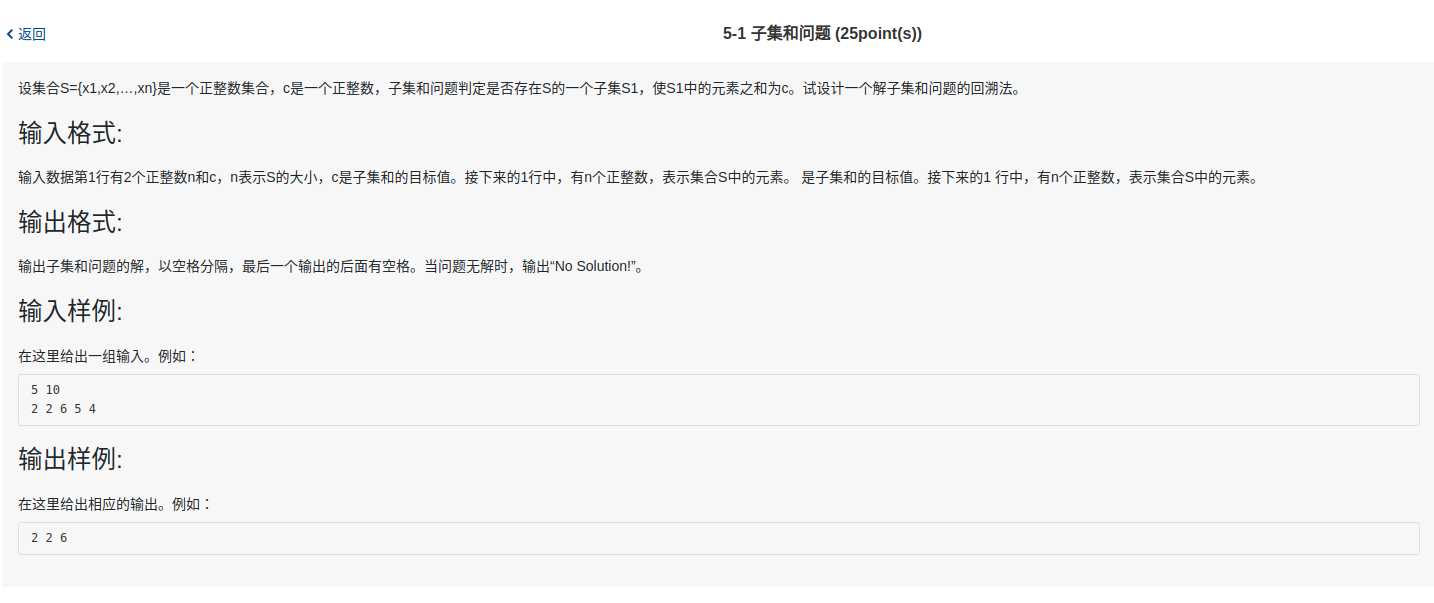
The way to solve the subset-sum problem will be introduced in the following sections to illustrate the algorithm. Detailed info is shown below in 7. Materials. Assume that the sub-set is
\[\{2\ 2\ 6\ 5\ 4\}\]
and the target sum is 10. Basically our task is to choose numbers in the given set to make the sum of numbers selected from the set is equal to the target sum.
Every solution in the back track algorithm is represented in the form of a set. And all of the solutions construct a solution space. For the subset-sum problem here, the solution space is:
\[\{0\ 0\ 0\ 0\ 0\}\]
\[\{1\ 0\ 0\ 0\ 0\}\]
\[\{0\ 1\ 0\ 0\ 0\}\]
\[ \vdots \]
\[\{1\ 1\ 1\ 1\ 0\}\]
\[\{1\ 1\ 1\ 1\ 1\}\]
Each digit in the set indicates if the number is selected. There are 5 numbers in the set to be chosen, each number may or may not be chosen, 2 status in other words. Thus the total number of solutions for the problem is
\[2^5 = 32\]
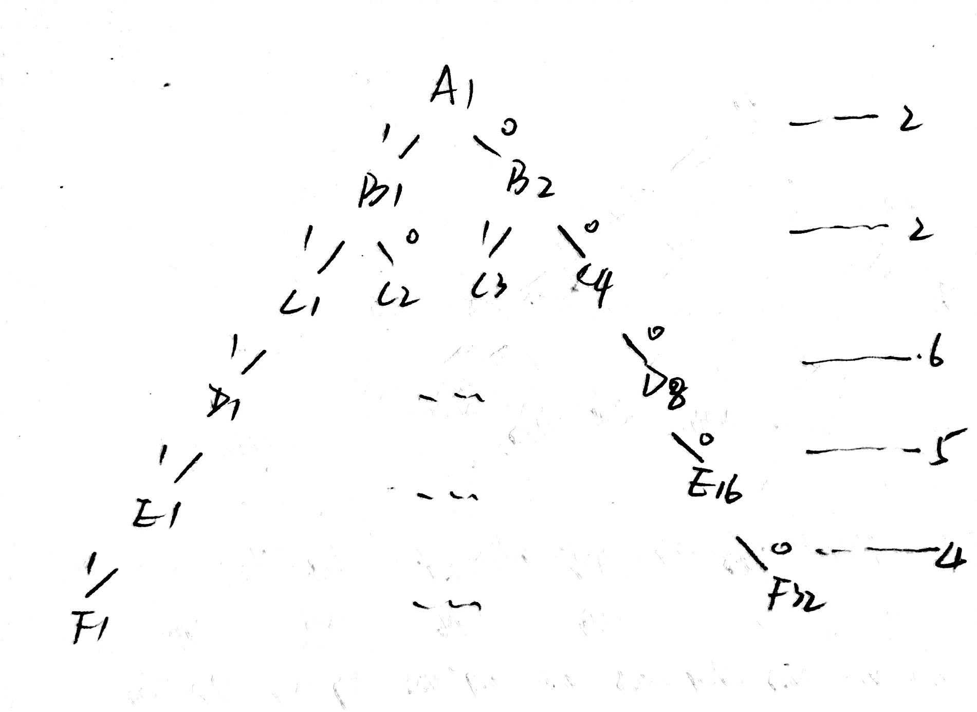
Generally the solution space is represented as a tree. Each edge of the tree represents a decision. For the problem here each edge represents if a specified number in the set is chosen. For the first number 2 there are two possible actions: choosing it or not choosing it. Thus there are two edges between the first and second layer in the tree. Let‘s say the edge on the left hand side denotes that the number is chosen, and the one on the right hand side denotes not choosing the number. And since there are two edges, there are two nodes in the second layer. Each node in the tree indicates the status after the decision which is reflected by the edge is made. For the problem here the left child node stores the current sum after adding the first number, and the right child node stores the same status as the node in the first layer, as the first number is not chosen.

DFS is used to iterater over the tree. Thus the algorithm appears as the form of a recursive function.
void backTrack(int t) {
  if (currentSum == c) {
    some operations
  } else if (t > n) {
    return;
  } else {
    some operations
    }
  }
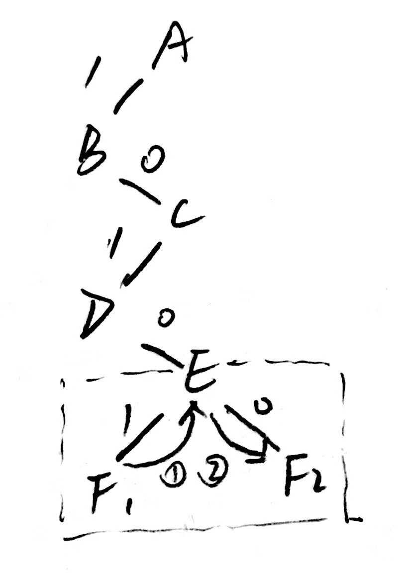
}Let‘s say now we get a solution \(\{1, 0, 1, 0, 1\}\) by going though related edges in the tree with the process described above. The current solution may not be the optimal solution. We should compare it with the optimal solution, and if the current one is better, replace it with the original optimal one. The solution now, however, may not be the optimal one since we have not gone through the whole solution space or the whole tree. To make it we should reset the status to that of the parent node of the current node. This is called back tracking, and it‘s exactly where the name of the algorithm comes from. Below the image shows the process.
the code related to the back tracking will be like
currentSum += S[t];
numbers[t] = 1;  // numbers[] stores the status (whether a specified number is chosen)

backTrace(t + 1);  // chooses the number, and evaluates the left child

currentSum -= S[t];  // back tracking
numbers[t] = 0;  // back tracking

backTrace(t + 1);  // does not choose the number, and evaluate the right child
There are generally two types of solution set tree. One is called subset tree and the other is called permutation tree. Solutions of a subset tree is about choosing some of the elements in the data set, meaning that some of the elements in the set can be abandoned, while those of a permutation tree is about reordering the elements in the data set to make the final result optimal, and all elements in the set should be kept.
There are two pruning functions used to avoid evaluating all solutions, enabling the algorithm to have a relatively good time complexity: the constraint function and the bound function.
The constraint function is used to avoid evaluating solutions that don‘t satisfied the requirement of the problem.
For the problem here, when the current sum is greater than the target sum. we need not consider the remaining numbers in the set anymore.
Say that the current sum is 13 which comes from
\[\{1\ 0\ 1\ 1\ ?\}\]
? means that we have not decided if the number 4 should be chosen. Now since the current sum is greater than 10, we need not consider if 4 should be chosen. What‘s reflected in the tree is that we need not consider the sub trees taking the nodes storing the status after choosing 5 as their root.
So the code now is
void backTrack(int t) {
  if (currentSum == c) {
    some operations
  } else if (t > n) {
    return;
  } else {
    if (currentSum <= c) {
      currentSum += S[t];
      numbers[t] = 1;  // numbers[] stores the status (whether a specified number is chosen)

      backTrace(t + 1);  // chooses the number, and evaluates the left child

      currentSum -= S[t];  // back tracking
      numbers[t] = 0;  // back tracking
    }

    backTrace(t + 1);  // does not choose the number, and evaluate the right child
  }
}
the condition representing the constraint function can also be written as a real function
bool constraint() {
  if (currentSum) <= c) {
    return true;
  } else {
    return false;
  }
}
and the code will be like
void backTrack(int t) {
  if (currentSum == c) {
    some operations
  } else if (t > n) {
    return;
  } else {
    if (constraint()) {
      currentSum += S[t];
      numbers[t] = 1;  // numbers[] stores the status (whether a specified number is chosen)

      backTrace(t + 1);  // chooses the number, and evaluates the left child

      currentSum -= S[t];  // back tracking
      numbers[t] = 0;  // back tracking
    }

    backTrace(t + 1);  // does not choose the number, and evaluate the right child
  }
}The bound function is used to avoid considering solutions that when their leaves, reflected in the tree, are reached, meaning that the solutions are completely constructed, the solutions will not be the ones we want..
For the problem here let‘s say we‘ve chosen some numbers and add them up. And if the sum is less than the target sum even after we add the remaining numbers to the current number, we need not consider the related solutions.
Say we now have a current sum of 0 which comes from
\[\{0\ 0\ 0\ ?\ ?\}\]
And the sum will be 9 after we add up all of the remaining numbers, 5 and 4 here. Since it is less than the target sum, we need not consider the solutions
\[\{0\ 0\ 0\ 0\ 0\}\]
\[\{0\ 0\ 0\ 0\ 1\}\]
\[\{0\ 0\ 0\ 1\ 0\}\]
\[\{0\ 0\ 0\ 1\ 1\}\]
What‘s reflected in the tree is that we need should consider the sub trees whose parent is the node storing the status after not choosing 6.
the bound function will be like
int bound(int t) {
  int bound = 0;
  for (int i = t; i <= n; i++) {
    bound += numbers[i];  // numbers[] stores given numbers
  }

  return bound;
}
and the code now is
void backTrack(int t) {
  if (currentSum == c) {
    some operations
  } else if (t > n) {
    return;
  } else {
    if (constraint()) {
      currentSum += S[t];
      numbers[t] = 1;  // numbers[] stores the status (whether a specified number is chosen)

      backTrace(t + 1);  // chooses the number, and evaluates the left child

      currentSum -= S[t];  // back tracking
      numbers[t] = 0;  // back tracking
    }

    if (currentSum + bound(t) >= c) {
      backTrace(t + 1);  // does not choose the number, and evaluate the right child
    }
  }
}According to the analysis above it‘s not hard to work out the general structure of the algorithm, as follows
void backTrack(int t) {  // t: the node keeping status after making some decisions
  if (t > n) {  // n: number of the data set
    if (the current solution is better than the original one) {
      assign the current solution to the original one or
      perform some other operations.
    } else {
      for (int i = 1; i <= n; i++) {  // considers all possible status of the current value
        if (constraint(t) && bound(t)) {
          back tracking

          backTrack(t + 1);

          back tracking
        }
      }
    }
  }
}The first question of the practice this time is the 0-1 knap sack problem. A strict bound function should be used to decrease the time complexity, or the running time will be longer than required. We worked for a pretty long time to solve it and finally found there was a mistake in the condition of an if statement evaluating if the bound is satisfied. The second problem can be solved using a permutation tree. I‘m not pretty familiar with this kind of tree and Yang Yizhou found the way to solve.

references:
[1] 王晓东. 计算机算法设计与分析. 北京: 电子工业出版社, 2018.
Back Tracking and the Subset-Sum Problem
标签:OLE task png node reflect this origin statement root
原文地址:https://www.cnblogs.com/Chunngai/p/12067033.html