标签:other regress length practice targe express name auto expect
Gaussian processes are the extension of multivariate Gaussians to infinite-size collections real valued variables. In particular, this extension will allow us to think of Gaussians processes as distributions not just over random vectors but in fact distribution over random functions.
A gaussian process is completely specified by its mean function $m(\cdot)$ and covariance function $k(\cdot,\cdot)$. if for any finite set of elements $x_1, \cdot, x_m \in \mathcal{X}$, the associated finite set of random variables $f(x_1), \cdots, f(x_m)$ have distribution:
\begin{equation} \left [ \begin{array}{c} f(x_1) \\ \vdots \\ f(x_m) \end{array} \right ] \sim \mathcal N \left ( \left [ \begin{array}{c} m(x_1) \\ \vdots \\ m(x_m) \end{array} \right ] , \left [ \begin{array}{ccc} k(x_1,x-1) & \cdots & k(x_1,x_m)\\ \vdots & \ddots & \vdots \\ k(x_m, x_1) & \cdots & k(x_m, x_m) \end{array}\right ] \right ) \end{equation}
we denote this using the notation
$$ f(\cdot) \sim \mathcal{GP}(m(\cdot), k(\cdot, \cdot)) $$
Observe that the mean function and covariance function are aptly name since the above property imply that
$$ m(x) = \mathbb E[x] $$
$$ k(x, x’) = \mathbb E[(x-m(x))(x’-m(x’))] $$
for any $x, x’ \in \mathcal X$
In order to get a proper Gaussian processes, for any set of element $x_1, \cdots, x_m \in \mathcal{X}$, the kernel matrix
\begin{equation} K(X,X) = \left [\begin{array}{ccc} k(x_1,x_1) & \cdots & k(x_1,x_m)\\ \vdots & \ddots & \vdots \\ k(x_m, x_1) & \cdots & k(x_m, x_m) \end{array} \right ] \end{equation}
is a valid covariance matrix corresponding to some multivariate Gaussian distribution. A standard results in probability theory states that this true provided that $K$ is positive semi-definite.
A simple example of Gaussian process can be obtained from our Bayesian linear regression model $f(x)=\phi(x)^T w$ with prior $w \sim \mathcal N(0, \Sigma_p)$. we have for the mean and covariance
\begin{eqnarray} \mathbb E[f(x)] &=& \phi(x)^T \mathbb E[w] \\ \mathbb E[(f(x)-0)(f(x’)-0)] &=& \phi(x)^T \mathbb E[ww^T] \phi(x’) = \phi(x)^T\Sigma_p \phi(x’) \end{eqnarray}
Thus $f(x)$ and $f(x’)$ are jointly Gaussian distribution with zero mean and covariance given by $\phi(x)^T\Sigma_p \phi(x’)$
The square exponential kernel function, defined as
\begin{equation} k_{SE}(x, x’) = \text{exp} (-\frac{1}{2l^2} || x-x’ ||^2 ) \label{SE_kernel} \end{equation}
with parameter $l$ define the characteristic length-scale.
In our example, since we use a zero-mean Gaussian process, we would expect that for the function value from our Gaussian process will tend to be distribute around zero. Furthermore, for any pair of $x,x’ \in \mathcal X$.
a. $f(x)$ and $f(x’)$ will tend to have high covariance $x$ and $x’$ are “nearby” in the input space. (i.e. $||x-x’||=|x-x’| \approx 0$, so $\text{exp}(-\frac{1}{2l^2} || x-x’ ||^2 ) \approx 1 $.
b. $f(x)$ and $f(x’)$ will tend to have low covariance when $x$ and $x’$ are “far apart”. (i.e. $||x-x’||=|x-x’| \gg 0$, so $\text{exp}(-\frac{1}{2l^2} || x-x’ ||^2 ) \approx 0 $.
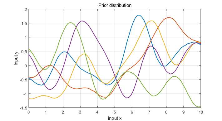
The specification of the covariance function implies a distribution over functions. To see this, we can draw samples from the distribution of functions evaluate at any number of input points, $X^*$ and write out the corresponding covariance matrix using (\ref{SE_kernel}). Then we generate a random Gaussian vector with covariance matrix
$$ f_* \sim \mathcal N(0, K(X_*, X_*)) $$
and plot the generated values as a function of the inputs
Let $S=\{(x^{(i)}, y^{(i)})\}_{i=1}^{n}$ be a training set of i.i.d. examples from some unknow distribution. In the Gaussian processes regression model.
$$ y = f(x) + \varepsilon $$
where the $\varepsilon$ are i.i.d. “noise” variables with independent $\mathcal N(0, \sigma_n^2)$ distribution Like in Bayesian linear regression, we also assume a prior distribution over functions $f(\cdot)$; in particular, we assume a zero-mean Gaussian process prior,
$$ f(\cdot) \sim \mathcal{GP} (0, k(\cdot,\cdot)) $$
for some valid covariance function $k(\cdot,\cdot)$.
The joint distribution of the training output, $f$ and the test output $f_*$ according to the prior is
\begin{equation} \left [ \begin{array}{c} f \\ f_* \end{array} \right ] \sim \mathcal N(0, \left [ \begin{array}{cc} K(X,X) & K(X, X_*) \\ K(X_*, X) & K(X_*, X_*) \end{array} \right ]) \end{equation}
Corresponding to condition the joint Gaussian prior distribution on the observations to give the joint posterior distribution
\begin{eqnarray} f_* | X_*, X, f \sim & \mathcal N & ( K(X_*,X) K(X,X)^{-1}f \nonumber \\ & & K(X_*, X_*) - K(X_*,X) K(X,X)^{-1}K(X, X_*) ) \end{eqnarray}
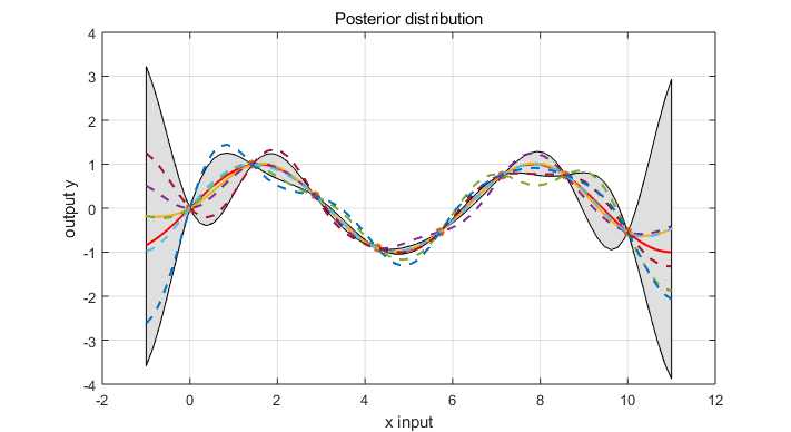
https://github.com/elike-ypq/Gaussian_Process/blob/master/Gassian_regression_no_noise.m
The prior on the noisy observations becomes
$$ cov(y_p,y_q) = k(x_p,x_q) + \sigma_n^2 \delta_{pq} \qquad \text{or} \qquad cov(y) = K(X,X) + \sigma_n^2 I $$
where $\delta_{pq}$ is Kronecker delta which is one iff $p=q$ and zero otherwise. We can rewrite the joint distribution of observed target values and the function values at the test location under the prior as
\begin{equation} \left [ \begin{array}{c} y \\ f_* \end{array} \right ] \sim \mathcal N(0, \left [ \begin{array}{cc} K(X,X) + \sigma_n^2 I & K(X, X_*) \\ K(X_*, X) & K(X_*, X_*) \end{array} \right ]) \end{equation}
Deriving the conditional distribution, we arrive at the key predictive equation for Gaussian process regression
\begin{equation} f_* | X, y, X_* \sim \mathcal N(\bar{f_*}, cov(f_*)) \end{equation}
where
\begin{eqnarray} \bar{f_*} &=& \mathbb E[f_* | X, y, X_* ] = K(X_*,X)[K(X,X)+\sigma_n^2 I]^{-1} y \\ cov(f_*) &=& K(X_*,X_*) – K(X_*,X) [K(X,X)+\sigma_n^2 I]^{-1}K(X,X_*) \end{eqnarray}
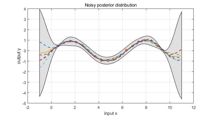
https://github.com/elike-ypq/Gaussian_Process/blob/master/Gassian_regression_with_noise.m
We can very simple compute the predictive distribution of test targets $y_*$ by adding $\sigma_n^2 I$ to the variance in the expression for $cov(f_*)$.
It is common but by no means necessary to consider GPs with a zero mean function. The use of a explicit basis functions is a way to specify a none zero mean over functions.
Using a fixed (deterministic) mean function $m(x)$ is trivial: simply apply the usual zero mean GP to the difference between the observations and the fixed mean function. With
$$ f(x) \sim \mathcal N(m(x), k(x,x’)) $$
the prediction mean becomes
$$ \bar{f_*} = \mathbb E[f_* | X, y, X_* ] = m(X_*) + K(X_*,X)[K(X,X)+\sigma_n^2 I]^{-1} (y-m(x)) $$
$$ cov(f_*) = K(X_*,X_*) – K(X_*,X) [K(X,X)+\sigma_n^2 I]^{-1}K(X,X_*) $$
However, in practice it can often be difficult to specify a fixed mean function. In many case, it may more convenient to specify a few fixed basis function, whose coefficients, $\beta$, are to be inferred from the data. Consider
\begin{equation} g(x) = f(x) + h(x)^T \beta \qquad \text{where} \qquad f(x) \sim \mathcal{GP} (0, k(x,x’)) \label{GP_e1}\end{equation}
here $f(x)$ is a zero mean GP, $h(x)$ are a set of fixed basis functions, and $\beta$ are additional parameters. When fitting the model, one could optimize over parameters $\beta$ jointly with the hyperparameter of the covariance function. Alternatively if we take the prior on $\beta$ to Gaussian, $\beta \sim \mathcal N(b, B)$, we can also integrate out this parameter. we obtain another GP
\begin{equation} g(x) \sim \mathcal{GP} (h(x)^Tb, k(x,x’)+ h(x)^T B h(x)) \label{GP_e2}\end{equation}
now with an added contribution in the covariance function caused by uncertainty in the parameters of the mean. Prediction are made by plugging the mean and covariance functions of $g(x)$ into (\ref{GP_e1}) and (\ref{GP_e2}). After rearranging, we obtain
\begin{eqnarray} \bar{g_*} &=& H_*^T\bar{\beta} + K(X_*,X)[K(X,X)+\sigma_n^2 I]^{-1} (y- H^T\bar{\beta}) = \bar{f_*} + R^T \bar{\beta} \\ cov(g_*) &=& cov(f_*) + R^T(B^{-1}+H K_y^{-1} H^T)^{-1} R \end{eqnarray}
where the $H$ matrix collects the $h(x)$ vectors for all training cases, $\bar{\beta} = (B^{-1}+ H K_y^{-1} H^T)^{-1} (H K_y^{-1}y + B^{-1} b )$, and $R = H_* – HK_y^{-1}H_*$
标签:other regress length practice targe express name auto expect
原文地址:https://www.cnblogs.com/eliker/p/11317738.html