标签:import splay ast self utf-8 rac lin rand 梯度
关键词:线性回归; linear Regression.
根据李航的归纳,机器学习模型有三要素,分别是:模型、策略和算法。为了简单好记,本文认为,在线性回归问题中,模型、策略和算法可以做如下简记:
模型 = 模型
策略 = 损失函数 + 优化目标
算法 = 解析解/数值计算方法 = 梯度下降方法
假设输出变量 \(\hat{y}\) 与输入变量 \(x_1\) 和 \(x_2\) 的关系为:
\[ \hat{y} = \hat{w_1} x_1 + \hat{w_2} x_2 + \hat{b} \]
建立上述模型的目的是为要拟合如下线性关系:
\[ y = w_1 x_1 + w_2 x_2 + b \]
设模型的损失函数为平方损失:
\[ L(\hat{w_1}, \hat{w_2}, \hat{b}) = \frac{1}{n} \sum_{i=1}^{n} L^{(i)}(\hat{w_1}, \hat{w_2}, \hat{b}) = \frac{1}{n} \sum_{i=1}^{n} \frac{1}{2}(\hat{y}^{(i)} - y^{(i)})^2 \]
目标函数为:
\[ w_1^*, w_2^*, b^* = \mathop{\arg\min}_{w_1, w_2, b} \ L(\hat{w_1}, \hat{w_2}, \hat{b}) \]
采用梯度下降方法更新参数的公式如下:
\[ \hat{w_1} = \hat{w_1} - \eta\frac{\partial{L}}{\partial{\hat{w_1}}} \\hat{w_2} = \hat{w_2} - \eta\frac{\partial{L}}{\partial{\hat{w_2}}} \\hat{b} = \hat{b} - \eta\frac{\partial{L}}{\partial{\hat{b}}} \]
为了方便理解,下面借助于复合函数求导法则将 \(\frac{\partial L}{\partial w_1}\) , \(\frac{\partial L}{\partial w_1}\) 和 \(\frac{\partial L}{\partial w_1}\) 分别展开:
\[ \begin{align} \frac{\partial L}{\partial \hat{w_1}} & = \frac{\partial \frac{1}{2} (\hat{y}-y)^2}{\partial \hat{y}} \cdot \frac{\partial \hat{y}}{\partial \hat{w_1}} \& = \frac{1}{2} \cdot 2 \cdot (\hat{y} - y) \cdot x_1 \& = (\hat{y} - y) \cdot x_1 \\frac{\partial L}{\partial \hat{w_2}} &= (\hat{y} - y) \cdot x_2 \\frac{\partial L}{\partial \hat{b}} &= \hat{y} - y \end{align} \]
模型参数在整个数据集上的更新公式如下:
\[ \hat{w_1} = \hat{w_1} - \frac{\eta}{n}\sum_{i\in{n}}(\hat{y}^{(i)} - y^{(i)})x_{1}^{(i)} \\hat{w_2} = \hat{w_2} - \frac{\eta}{n}\sum_{i\in{n}}(\hat{y}^{(i)} - y^{(i)})x_{2}^{(i)} \\hat{b} = \hat{b} - \frac{\eta}{n}\sum_{i\in{n}}(\hat{y}^{(i)} - y^{(i)}) \]
本文选用小批量随机梯度下降(mini-batch Stochastic Gradient Descend)方法来优化模型,设每次取得的批量大小为 \(|\mathcal{B}|\),则模型的近似平均损失如下:
\[ L = \frac{1}{|\mathcal{B}|} \sum_{i=1}^{|\mathcal{B}|} \frac{1}{2}(\hat{y}^{(i)} - y^{(i)})^2 \]
采用了小批量随机梯度下降的 \(\frac{\partial L}{\partial w_1}\) , \(\frac{\partial L}{\partial w_1}\) 和 \(\frac{\partial L}{\partial w_1}\) 分别展开:
\[ \begin{align} \frac{\partial L}{\partial \hat{w_1}} & = \frac{\partial \frac{1}{|\mathcal{B}|} \sum_{i=1}^{|\mathcal{B}|} \frac{1}{2} (\hat{y}^{(i)}-y^{(i)})^2}{\partial \hat{w_1}} \& = \frac{1}{\mathcal{|B|}} \sum_{i=1}^{\mathcal{|B|}} (\hat{y}^{(i)} - y^{(i)}) x_{1}^{(i)} \\frac{\partial L}{\partial \hat{w_2}} & = \frac{1}{\mathcal{|B|}} \sum_{i=1}^{\mathcal{|B|}} (\hat{y}^{(i)} - y^{(i)}) x_{2}^{(i)} \\frac{\partial L}{\partial \hat{b}} & = \frac{1}{\mathcal{|B|}} \sum_{i=1}^{\mathcal{|B|}} (\hat{y}^{(i)} - y^{(i)}) \\end{align} \]
模型各个参数的更新方法如下:
\[ \hat{w_1} = \hat{w_1} - \frac{\eta}{\mathcal{|B|}} \sum_{i\in{\mathcal{B}}} (\hat{y}^{(i)} - y^{(i)}) x_{1}^{(i)} \\hat{w_2} = \hat{w_2} - \frac{\eta}{\mathcal{|B|}} \sum_{i\in{\mathcal{B}}} (\hat{y}^{(i)} - y^{(i)}) x_{2}^{(i)} \\hat{b} = \hat{b} - \frac{\eta}{\mathcal{|B|}} \sum_{i\in{\mathcal{B}}} (\hat{y}^{(i)} - y^{(i)}) \]
基于小批量梯度下降的线性回归:使用 Python3 实现
# coding=utf-8
import numpy as np
from matplotlib import pyplot as plt
def generate_data(w, b, sample_num):
feature_num = len(w)
w = np.array(w).reshape(-1, 1)
x = np.random.random(sample_num * feature_num).reshape(sample_num, feature_num)
eta = np.random.normal(size=(sample_num, 1))
y = np.matmul(x, w) + b + eta
return x, y
class LinearRegression:
def __init__(self, lr=0.001):
self.eta = lr
def fit(self, x, y, epochs=30, batch_size=32):
losses = list()
sample_num, feature_num = x.shape
self.w, self.b = np.random.normal(size=(feature_num, 1)), np.random.random()
batch_num = sample_num / batch_size if sample_num % batch_size == 0 else int(sample_num / batch_size) + 1
for epoch in range(epochs):
for batch in range(batch_num):
x_batch = x[batch*batch_size:(batch+1)*batch_size, :]
y_batch = y[batch*batch_size:(batch+1)*batch_size]
y_batch_pred = self.predict(x_batch)
error = y_batch_pred - y_batch
average_error = np.average(error)
self.b = self.b - self.eta * average_error
for i in range(feature_num):
gradient = error * x[:, i]
average_gradient = np.average(gradient)
self.w[i] = self.w[i] - self.eta * average_gradient
y_pred = self.predict(x)
error = y_pred - y
average_error = np.average(error)
loss = average_error * average_error / 2
print("[Epoch]%d [Loss]%f [w1]%.2f [w2]%.2f [b]%.2f" % (epoch, loss, self.w[0], self.w[1], self.b))
losses.append(loss)
return losses
def predict(self, x):
left = np.matmul(x, self.w)
y = left + b
return y
if __name__ == '__main__':
sample_num = 1000
w = [2.5, 1.3]
b = 1.8
x, y = generate_data(w, b, sample_num)
lr = LinearRegression(lr=0.001)
loss = lr.fit(x, y, epochs=300)
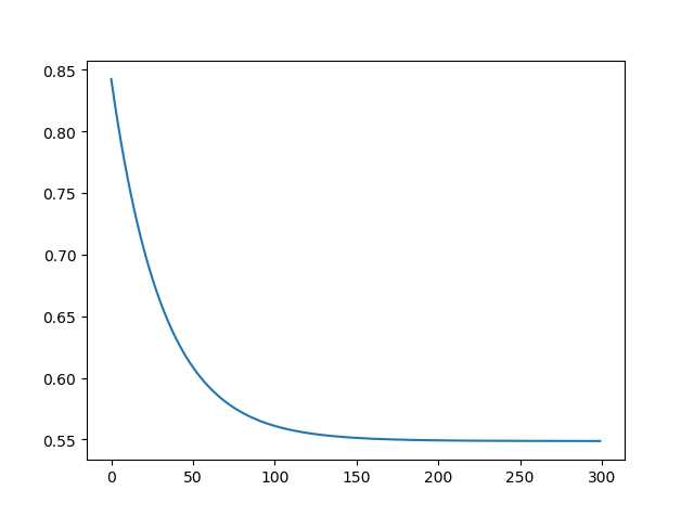
plt.plot(loss)
plt.show()
实验结果:
[Epoch]299 [Loss]0.548715 [w1]1.87 [w2]1.88 [b]2.40损失图像:
在本文中,我们有如下贡献:
通过实验,我们有如下结论:
标签:import splay ast self utf-8 rac lin rand 梯度
原文地址:https://www.cnblogs.com/fengyubo/p/12514427.html