Overview
- Time Series Analysis and Time Series Modeling are powerful forecasting tools
- A prior knowledge of the statistical theory behind Time Series is useful before Time series Modeling
- ARMA and ARIMA are important models for performing Time Series Analysis
Introduction
‘Time’ is the most important factor which ensures success in a business. It’s difficult to keep up with the pace of time. But, technology has developed some powerful methods using which we can ‘see things’ ahead of time. Don’t worry, I am not talking about Time Machine. Let’s be realistic here!
I’m talking about the methods of prediction & forecasting. One such method, which deals with time based data is Time Series Modeling. As the name suggests, it involves working on time (years, days, hours, minutes) based data, to derive hidden insights to make informed decision making.
Time series models are very useful models when you have serially correlated data. Most of business houses work on time series data to analyze sales number for the next year, website traffic, competition position and much more. However, it is also one of the areas, which many analysts do not understand.
So, if you aren’t sure about complete process of time series modeling, this guide would introduce you to various levels of time series modeling and its related techniques.
Table of Contents
- Basics – Time Series Modeling
- Exploration of Time Series Data in R
- Introduction to ARMA Time Series Modeling
- Framework and Application of ARIMA Time Series Modeling
Time to get started!
1. Basics – Time Series Modeling
Let’s begin from basics. This includes stationary series, random walks , Rho Coefficient, Dickey Fuller Test of Stationarity. If these terms are already scaring you, don’t worry – they will become clear in a bit and I bet you will start enjoying the subject as I explain it.
Stationary Series
There are three basic criterion for a series to be classified as stationary series :
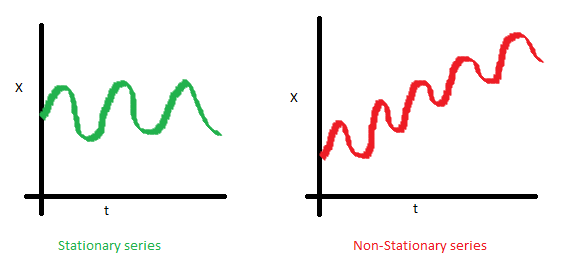
1. The mean of the series should not be a function of time rather should be a constant. The image below has the left hand graph satisfying the condition whereas the graph in red has a time dependent mean.
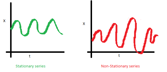
2. The variance of the series should not a be a function of time. This property is known as homoscedasticity. Following graph depicts what is and what is not a stationary series. (Notice the varying spread of distribution in the right hand graph)
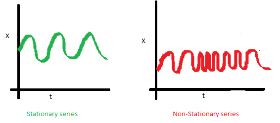
3. The covariance of the i th term and the (i + m) th term should not be a function of time. In the following graph, you will notice the spread becomes closer as the time increases. Hence, the covariance is not constant with time for the ‘red series’.
Why do I care about ‘stationarity’ of a time series?
The reason I took up this section first was that until unless your time series is stationary, you cannot build a time series model. In cases where the stationary criterion are violated, the first requisite becomes to stationarize the time series and then try stochastic models to predict this time series. There are multiple ways of bringing this stationarity. Some of them are Detrending, Differencing etc.
Random Walk
This is the most basic concept of the time series. You might know the concept well. But, I found many people in the industry who interprets random walk as a stationary process. In this section with the help of some mathematics, I will make this concept crystal clear for ever. Let’s take an example.
Example: Imagine a girl moving randomly on a giant chess board. In this case, next position of the girl is only dependent on the last position.
(Source: http://scifun.chem.wisc.edu/WOP/RandomWalk.html )
Now imagine, you are sitting in another room and are not able to see the girl. You want to predict the position of the girl with time. How accurate will you be? Of course you will become more and more inaccurate as the position of the girl changes. At t=0 you exactly know where the girl is. Next time, she can only move to 8 squares and hence your probability dips to 1/8 instead of 1 and it keeps on going down. Now let’s try to formulate this series :
X(t) = X(t-1) + Er(t)
where Er(t) is the error at time point t. This is the randomness the girl brings at every point in time.
Now, if we recursively fit in all the Xs, we will finally end up to the following equation :
X(t) = X(0) + Sum(Er(1),Er(2),Er(3).....Er(t))
Now, lets try validating our assumptions of stationary series on this random walk formulation:
1. Is the Mean constant ?
E[X(t)] = E[X(0)] + Sum(E[Er(1)],E[Er(2)],E[Er(3)].....E[Er(t)])
We know that Expectation of any Error will be zero as it is random.
Hence we get E[X(t)] = E[X(0)] = Constant.
2. Is the Variance constant?
Var[X(t)] = Var[X(0)] + Sum(Var[Er(1)],Var[Er(2)],Var[Er(3)].....Var[Er(t)])
Var[X(t)] = t * Var(Error) = Time dependent.
Hence, we infer that the random walk is not a stationary process as it has a time variant variance. Also, if we check the covariance, we see that too is dependent on time.
Let’s spice up things a bit,
We already know that a random walk is a non-stationary process. Let us introduce a new coefficient in the equation to see if we can make the formulation stationary.
Introduced coefficient : Rho
X(t) = Rho * X(t-1) + Er(t)
Now, we will vary the value of Rho to see if we can make the series stationary. Here we will interpret the scatter visually and not do any test to check stationarity.
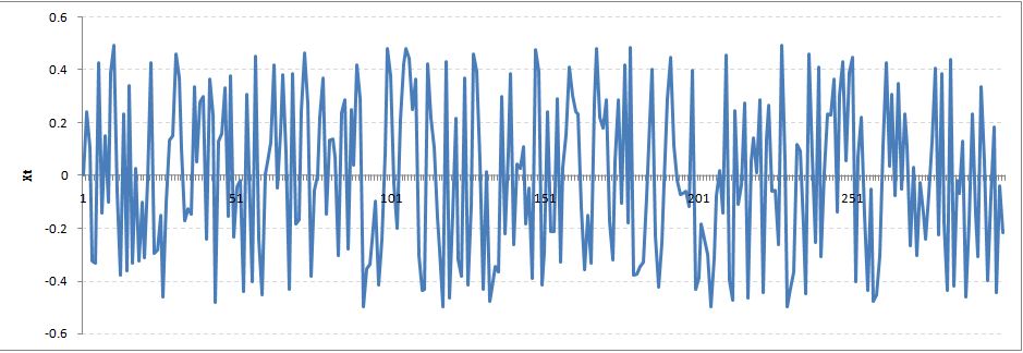
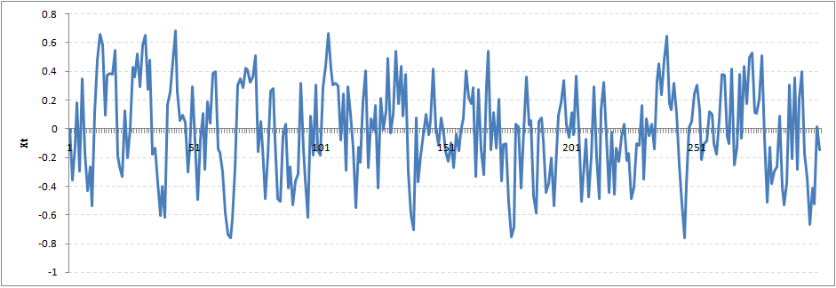
Let’s start with a perfectly stationary series with Rho = 0 . Here is the plot for the time series :
Increase the value of Rho to 0.5 gives us following graph :
You might notice that our cycles have become broader but essentially there does not seem to be a serious violation of stationary assumptions. Let’s now take a more extreme case of Rho = 0.9
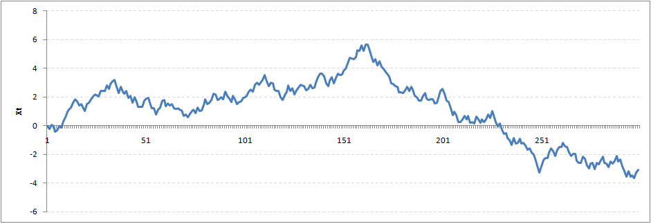
We still see that the X returns back from extreme values to zero after some intervals. This series also is not violating non-stationarity significantly. Now, let’s take a look at the random walk with rho = 1.
This obviously is an violation to stationary conditions. What makes rho = 1 a special case which comes out badly in stationary test? We will find the mathematical reason to this.
Let’s take expectation on each side of the equation “X(t) = Rho * X(t-1) + Er(t)”
E[X(t)] = Rho *E[ X(t-1)]
This equation is very insightful. The next X (or at time point t) is being pulled down to Rho * Last value of X.
For instance, if X(t – 1 ) = 1, E[X(t)] = 0.5 ( for Rho = 0.5) . Now, if X moves to any direction from zero, it is pulled back to zero in next step. The only component which can drive it even further is the error term. Error term is equally probable to go in either direction. What happens when the Rho becomes 1? No force can pull the X down in the next step.
Dickey Fuller Test of Stationarity
What you just learnt in the last section is formally known as Dickey Fuller test. Here is a small tweak which is made for our equation to convert it to a Dickey Fuller test:
X(t) = Rho * X(t-1) + Er(t)
=>  X(t) - X(t-1) = (Rho - 1) X(t - 1) + Er(t)
We have to test if Rho – 1 is significantly different than zero or not. If the null hypothesis gets rejected, we’ll get a stationary time series.
Stationary testing and converting a series into a stationary series are the most critical processes in a time series modelling. You need to memorize each and every detail of this concept to move on to the next step of time series modelling.
Let’s now consider an example to show you what a time series looks like.
2. Exploration of Time Series Data in R
Here we’ll learn to handle time series data on R. Our scope will be restricted to data exploring in a time series type of data set and not go to building time series models.
I have used an inbuilt data set of R called AirPassengers. The dataset consists of monthly totals of international airline passengers, 1949 to 1960.
Loading the Data Set
Following is the code which will help you load the data set and spill out a few top level metrics.
> data(AirPassengers)
 > class(AirPassengers)
 [1] "ts"
#This tells you that the data series is in a time series format
 > start(AirPassengers)
 [1] 1949 1
#This is the start of the time series
> end(AirPassengers)
 [1] 1960 12
#This is the end of the time series
> frequency(AirPassengers)
 [1] 12
#The cycle of this time series is 12months in a year
 > summary(AirPassengers)
 Min. 1st Qu. Median Mean 3rd Qu. Max.
 104.0 180.0 265.5 280.3 360.5 622.0
Detailed Metrics
#The number of passengers are distributed across the spectrum
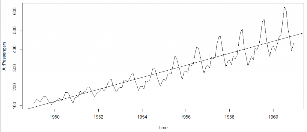
> plot(AirPassengers)
#This will plot the time series
>abline(reg=lm(AirPassengers~time(AirPassengers)))
# This will fit in a line
Here are a few more operations you can do:
> cycle(AirPassengers)
#This will print the cycle across years.
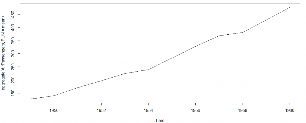
>plot(aggregate(AirPassengers,FUN=mean))
#This will aggregate the cycles and display a year on year trend
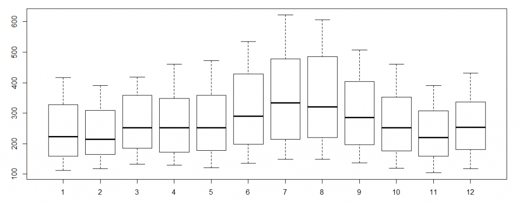
> boxplot(AirPassengers~cycle(AirPassengers))
#Box plot across months will give us a sense on seasonal effect
Important Inferences
- The year on year trend clearly shows that the #passengers have been increasing without fail.
- The variance and the mean value in July and August is much higher than rest of the months.
- Even though the mean value of each month is quite different their variance is small. Hence, we have strong seasonal effect with a cycle of 12 months or less.
Exploring data becomes most important in a time series model – without this exploration, you will not know whether a series is stationary or not. As in this case we already know many details about the kind of model we are looking out for.
Let’s now take up a few time series models and their characteristics. We will also take this problem forward and make a few predictions.
3. Introduction to ARMA Time Series Modeling
ARMA models are commonly used in time series modeling. In ARMA model, AR stands for auto-regression and MA stands for moving average. If these words sound intimidating to you, worry not – I’ll simplify these concepts in next few minutes for you!
We will now develop a knack for these terms and understand the characteristics associated with these models. But before we start, you should remember, AR or MA are not applicable on non-stationary series.
In case you get a non stationary series, you first need to stationarize the series (by taking difference / transformation) and then choose from the available time series models.
First, I’ll explain each of these two models (AR & MA) individually. Next, we will look at the characteristics of these models.
Auto-Regressive Time Series Model
Let’s understanding AR models using the case below:
The current GDP of a country say x(t) is dependent on the last year’s GDP i.e. x(t – 1). The hypothesis being that the total cost of production of products & services in a country in a fiscal year (known as GDP) is dependent on the set up of manufacturing plants / services in the previous year and the newly set up industries / plants / services in the current year. But the primary component of the GDP is the former one.
Hence, we can formally write the equation of GDP as:
x(t) = alpha * x(t – 1) + error (t)
This equation is known as AR(1) formulation. The numeral one (1) denotes that the next instance is solely dependent on the previous instance. The alpha is a coefficient which we seek so as to minimize the error function. Notice that x(t- 1) is indeed linked to x(t-2) in the same fashion. Hence, any shock to x(t) will gradually fade off in future.
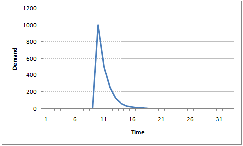
For instance, let’s say x(t) is the number of juice bottles sold in a city on a particular day. During winters, very few vendors purchased juice bottles. Suddenly, on a particular day, the temperature rose and the demand of juice bottles soared to 1000. However, after a few days, the climate became cold again. But, knowing that the people got used to drinking juice during the hot days, there were 50% of the people still drinking juice during the cold days. In following days, the proportion went down to 25% (50% of 50%) and then gradually to a small number after significant number of days. The following graph explains the inertia property of AR series:
Moving Average Time Series Model
Let’s take another case to understand Moving average time series model.
A manufacturer produces a certain type of bag, which was readily available in the market. Being a competitive market, the sale of the bag stood at zero for many days. So, one day he did some experiment with the design and produced a different type of bag. This type of bag was not available anywhere in the market. Thus, he was able to sell the entire stock of 1000 bags (lets call this as x(t) ). The demand got so high that the bag ran out of stock. As a result, some 100 odd customers couldn’t purchase this bag. Lets call this gap as the error at that time point. With time, the bag had lost its woo factor. But still few customers were left who went empty handed the previous day. Following is a simple formulation to depict the scenario :
x(t) = beta * error(t-1) + error (t)
If we try plotting this graph, it will look something like this :
Did you notice the difference between MA and AR model? In MA model, noise / shock quickly vanishes with time. The AR model has a much lasting effect of the shock.
Difference between AR and MA models
The primary difference between an AR and MA model is based on the correlation between time series objects at different time points. The correlation between x(t) and x(t-n) for n > order of MA is always zero. This directly flows from the fact that covariance between x(t) and x(t-n) is zero for MA models (something which we refer from the example taken in the previous section). However, the correlation of x(t) and x(t-n) gradually declines with n becoming larger in the AR model. This difference gets exploited irrespective of having the AR model or MA model. The correlation plot can give us the order of MA model.
Exploiting ACF and PACF plots
Once we have got the stationary time series, we must answer two primary questions:
Q1. Is it an AR or MA process?
Q2. What order of AR or MA process do we need to use?
The trick to solve these questions is available in the previous section. Didn’t you notice?
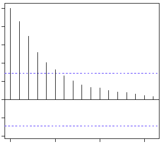
The first question can be answered using Total Correlation Chart (also known as Auto – correlation Function / ACF). ACF is a plot of total correlation between different lag functions. For instance, in GDP problem, the GDP at time point t is x(t). We are interested in the correlation of x(t) with x(t-1) , x(t-2) and so on. Now let’s reflect on what we have learnt above.
In a moving average series of lag n, we will not get any correlation between x(t) and x(t – n -1) . Hence, the total correlation chart cuts off at nth lag. So it becomes simple to find the lag for a MA series. For an AR series this correlation will gradually go down without any cut off value. So what do we do if it is an AR series?
Here is the second trick. If we find out the partial correlation of each lag, it will cut off after the degree of AR series. For instance,if we have a AR(1) series, if we exclude the effect of 1st lag (x (t-1) ), our 2nd lag (x (t-2) ) is independent of x(t). Hence, the partial correlation function (PACF) will drop sharply after the 1st lag. Following are the examples which will clarify any doubts you have on this concept :
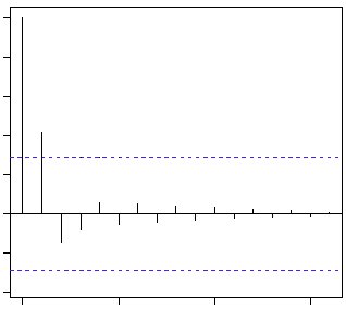
ACF PACF
The blue line above shows significantly different values than zero. Clearly, the graph above has a cut off on PACF curve after 2nd lag which means this is mostly an AR(2) process.
ACF PACF
Clearly, the graph above has a cut off on ACF curve after 2nd lag which means this is mostly a MA(2) process.
Till now, we have covered on how to identify the type of stationary series using ACF & PACF plots. Now, I’ll introduce you to a comprehensive framework to build a time series model. In addition, we’ll also discuss about the practical applications of time series modelling.
4. Framework and Application of ARIMA Time Series Modeling
A quick revision, Till here we’ve learnt basics of time series modeling, time series in R and ARMA modeling. Now is the time to join these pieces and make an interesting story.
Overview of the Framework
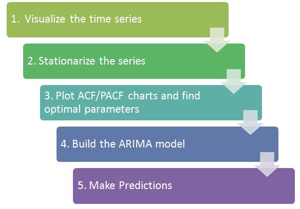
This framework(shown below) specifies the step by step approach on ‘How to do a Time Series Analysis‘:
As you would be aware, the first three steps have already been discussed above. Nevertheless, the same has been delineated briefly below:
Step 1: Visualize the Time Series
It is essential to analyze the trends prior to building any kind of time series model. The details we are interested in pertains to any kind of trend, seasonality or random behaviour in the series. We have covered this part in the second part of this series.
Step 2: Stationarize the Series
Once we know the patterns, trends, cycles and seasonality , we can check if the series is stationary or not. Dickey – Fuller is one of the popular test to check the same. We have covered this test in the first part of this article series. This doesn’t ends here! What if the series is found to be non-stationary?
There are three commonly used technique to make a time series stationary:
1. Detrending : Here, we simply remove the trend component from the time series. For instance, the equation of my time series is:
x(t) = (mean + trend * t) + error
We’ll simply remove the part in the parentheses and build model for the rest.
2. Differencing : This is the commonly used technique to remove non-stationarity. Here we try to model the differences of the terms and not the actual term. For instance,
x(t) – x(t-1) = ARMA (p , q)
This differencing is called as the Integration part in AR(I)MA. Now, we have three parameters
p : AR

d : I

q : MA
3. Seasonality : Seasonality can easily be incorporated in the ARIMA model directly. More on this has been discussed in the applications part below.
Step 3: Find Optimal Parameters
The parameters p,d,q can be found using ACF and PACF plots. An addition to this approach is can be, if both ACF and PACF decreases gradually, it indicates that we need to make the time series stationary and introduce a value to “d”.
Step 4: Build ARIMA Model
With the parameters in hand, we can now try to build ARIMA model. The value found in the previous section might be an approximate estimate and we need to explore more (p,d,q) combinations. The one with the lowest BIC and AIC should be our choice. We can also try some models with a seasonal component. Just in case, we notice any seasonality in ACF/PACF plots.
Step 5: Make Predictions
Once we have the final ARIMA model, we are now ready to make predictions on the future time points. We can also visualize the trends to cross validate if the model works fine.
Applications of Time Series Model
Now, we’ll use the same example that we have used above. Then, using time series, we’ll make future predictions. We recommend you to check out the example before proceeding further.
Where did we start ?
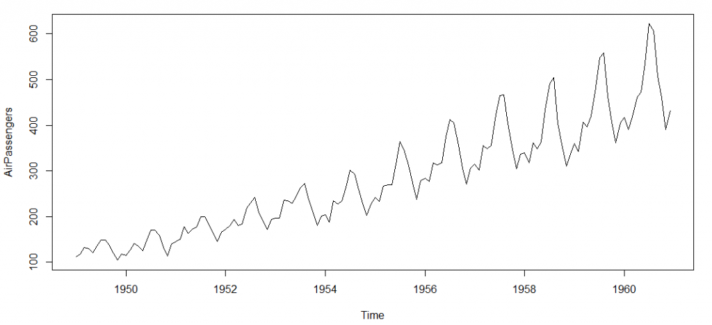
Following is the plot of the number of passengers with years. Try and make observations on this plot before moving further in the article.
Here are my observations :
1. There is a trend component which grows the passenger year by year.
2. There looks to be a seasonal component which has a cycle less than 12 months.
3. The variance in the data keeps on increasing with time.
We know that we need to address two issues before we test stationary series. One, we need to remove unequal variances. We do this using log of the series. Two, we need to address the trend component. We do this by taking difference of the series. Now, let’s test the resultant series.
adf.test(diff(log(AirPassengers)), alternative="stationary", k=0)
Augmented Dickey-Fuller Test
data: diff(log(AirPassengers))
 Dickey-Fuller = -9.6003, Lag order = 0,
 p-value = 0.01
 alternative hypothesis: stationary
We see that the series is stationary enough to do any kind of time series modelling.
Next step is to find the right parameters to be used in the ARIMA model. We already know that the ‘d’ component is 1 as we need 1 difference to make the series stationary. We do this using the Correlation plots. Following are the ACF plots for the series :
#ACF Plots
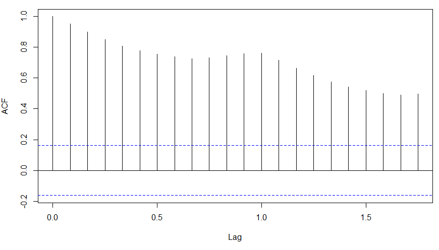
acf(log(AirPassengers))
What do you see in the chart shown above?
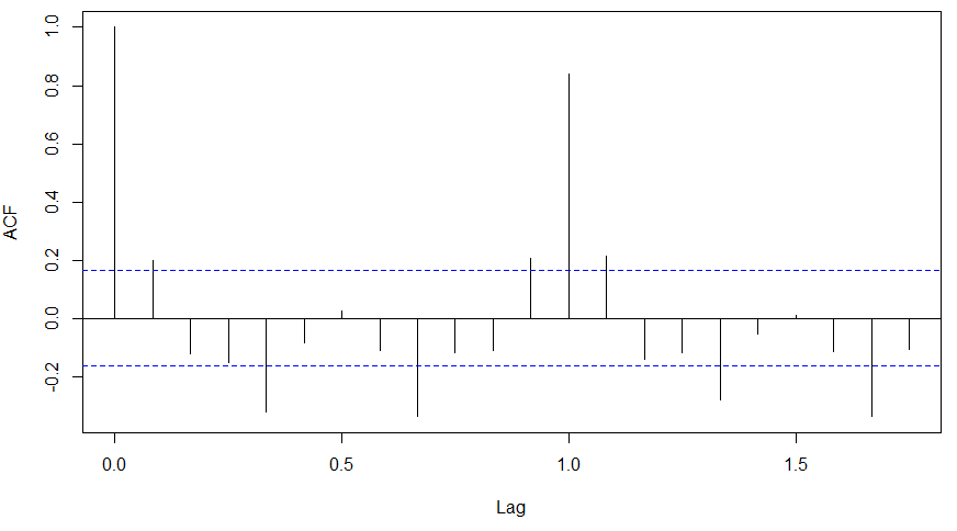
Clearly, the decay of ACF chart is very slow, which means that the population is not stationary. We have already discussed above that we now intend to regress on the difference of logs rather than log directly. Let’s see how ACF and PACF curve come out after regressing on the difference. [stextbox id="grey"]
acf(diff(log(AirPassengers)))
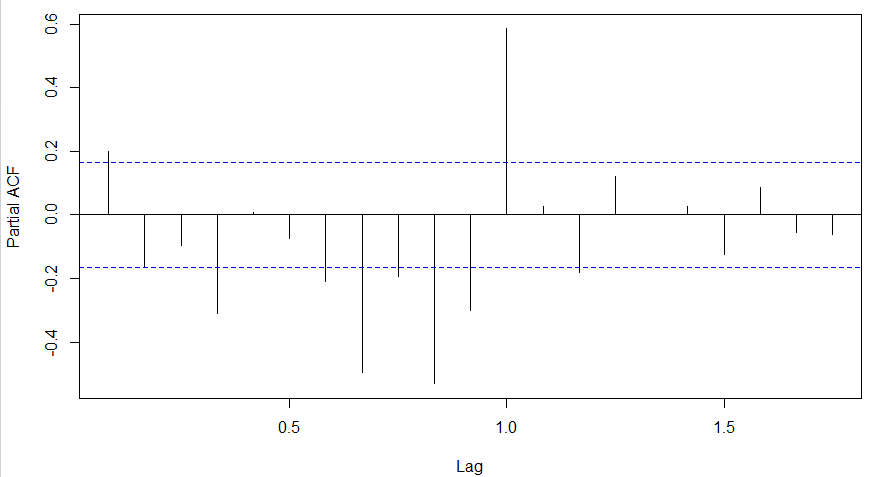
pacf(diff(log(AirPassengers)))
Clearly, ACF plot cuts off after the first lag. Hence, we understood that value of p should be 0 as the ACF is the curve getting a cut off. While value of q should be 1 or 2. After a few iterations, we found that (0,1,1) as (p,d,q) comes out to be the combination with least AIC and BIC.
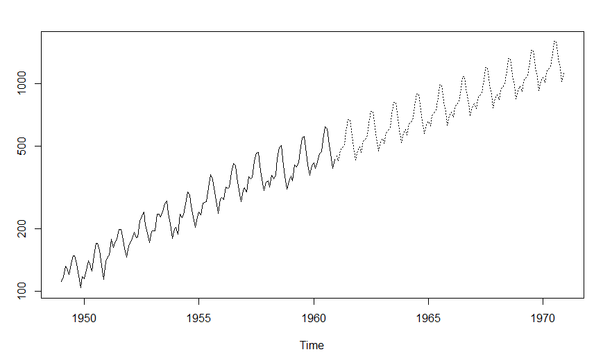
Let’s fit an ARIMA model and predict the future 10 years. Also, we will try fitting in a seasonal component in the ARIMA formulation. Then, we will visualize the prediction along with the training data. You can use the following code to do the same :
(fit <- arima(log(AirPassengers), c(0, 1, 1),seasonal = list(order = c(0, 1, 1), period = 12)))
pred <- predict(fit, n.ahead = 10*12)
ts.plot(AirPassengers,2.718^pred$pred, log = "y", lty = c(1,3))


