标签:xpl lock ddr unicode 大型 直接 val 快速 读取
数据来源:https://www.kaggle.com/wendykan/lending-club-loan-data
数据描述:LendingClub是一家美国P2P借贷公司,总部位于加利福尼亚州旧金山。这是第一个对等网络贷款人登记其产品为证券与证券交易委员会(SEC),并在二级市场上提供贷款交易。LendingClub是世界上最大的点对点借贷平台。这些文件包含 LENGDING CLUB 公司 2007-2015 年间发放的所有贷款的完整贷款数据,包括当前贷款状态(“当前”,“延迟”,“已全额付款”等)和最新付款信息。该文件是约226万个观测值和145个字段的矩阵,字段包括信用评分,财务查询数量,包括邮政编码的地址,状态以及收款等信息。 数据字段字典在单独的文件中提供。
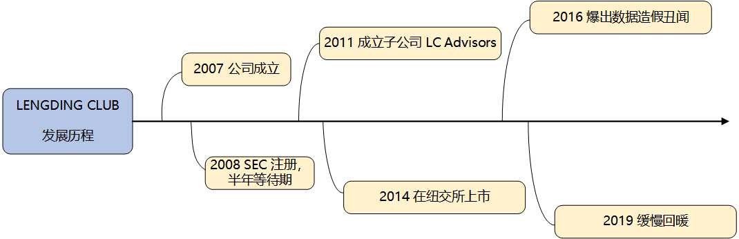
图1 Lending Club 发展历程
2007年,Lending Club 成立,主营业务是为市场提供P2P贷款的平台中介服务。与已运营两年的占据美国 P2P 市场最大份额的 Prosper 形成差异化竞争。初期为了对平台进行第一轮推广,希望利用社交网络发现潜在客户,与 Facebook 合作,但其用户大部分为年轻人,不具备贷款投资能力,这样的合作为其带来了巨大的点击率但没有带来足够的贷款量增长。9月份,Lending Club 对社交方式进行调整,投向更多社交平台以外的用户,自此快速发展。
2008年3月,美国证券交易委员会 SEC 将 Lending Club 平台出手的票据认定为票据,需要平台对其进行注册。4月7日,进入半年的注册等待期。完成 SEC 注册后,为了增加贷款投资的流动性,Lending Club 与经济交易商 FOLIOfn (平台运营者,只撮合双方交易,不参与做市)合作建立了二级交易平台。二级交易平台的建立,使投资者持有的收益权凭证能够和股票一样在二级市场上交易,迅速变现。
2011年11月,Lending Club 创办了全资子公司 LC Advisors,LC Advisors是一家 SEC 认可的投资咨询公司,专门负责管理 Lending Club 大型投资者的投资。
2014年12月,Lending Club 在纽交所上市,成为当年最大的科技股IPO。
2015年2月3日起,阿里巴巴宣布将和 Lending Club 合作,为向中国供应商采购商品的美国小企业提供贷款。
2015年2月10日,LC 宣布和美国 200 家银行达成合作关系。BancAlliance 是一个由资产2亿到100亿美元不等的200家社区银行组成的联盟。
2016年5月9日,Lending Club 首席执行官 Renaud Laplanche 宣布辞职。在一场内部调查中,董事会发现公司存在向机构投资者舞弊,数据造假等问题。另外 Renaud Laplanche 还未能尽到披露义务,说明自己已持有一家投资基金的股份,并主导了Lending Club对这家公司的投资。
2016-2018,Lending Club 股价下跌,治理丑闻,此时,其他许多 P2P 公司也遇到了困难。
2019年12月,执行官Valerie Kay指出,LendingClub已通过一个名为``Scale‘‘的新项目将重点转移到机构投资者以及其传统的点对点贷款,该项目专注于提供代表性贷款样本而不是个人贷款。LendingClub在2018年的年度贷款发放额已增长至108亿美元。
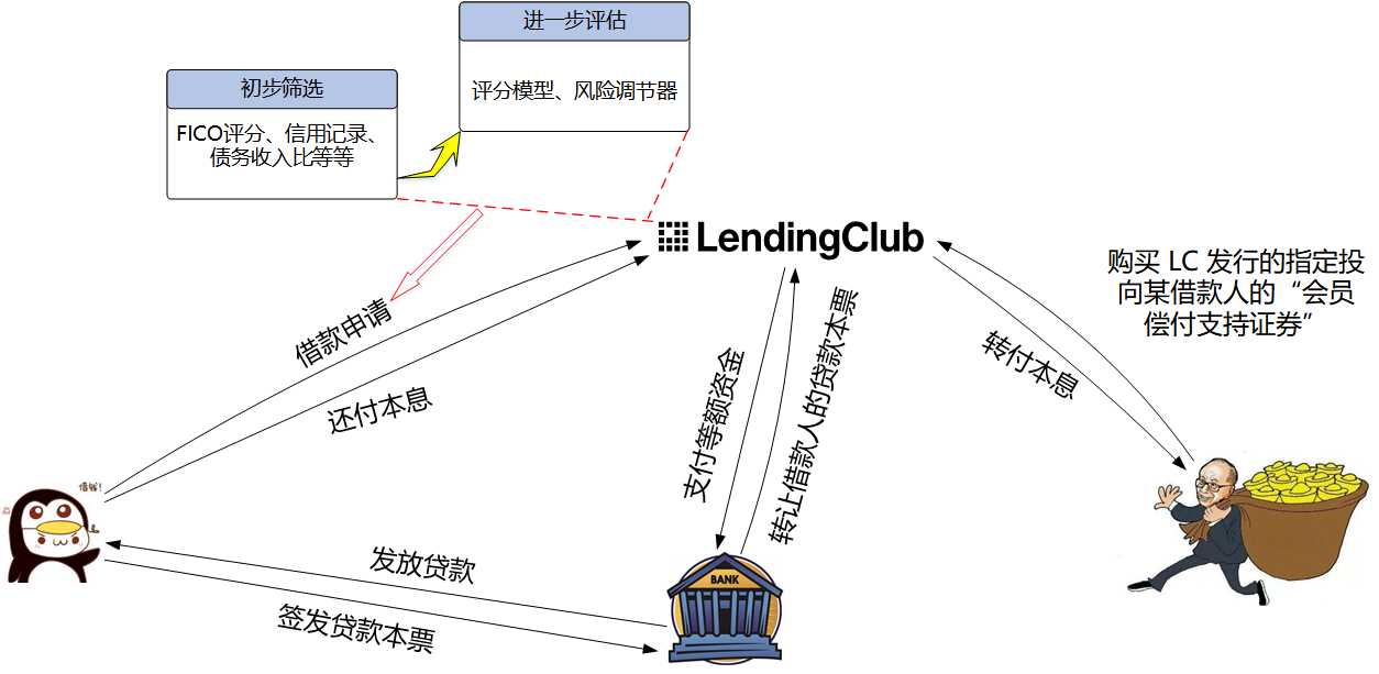
图2 Lending Club 贷款业务过程
贷款人希望在 Lending Club 平台借款时,首先需要在平台上发布借款请求,请求中包含很多有关借款人的信息,如借款人的 FICO 分数,信用级别,借款目的,借款期限,借款金额,借款进度,借款人收入,月还款额,债务收入比,就业状况,信用记录等。但是,投资者和借款人在 Lending Club 上都是匿名的,双方在交易过程中并不清楚对方的真实身份,这正是 Lending Club 要为客户保护的。投资人(出借者)可以浏览借款列表选中自己认可的借款人来投资,也可以根据自己的偏好设定投资组合。待各个投资者承诺的出借金额的累加达到了借款人所需要的总金额,或自借款请求列表发布日起已累计达 14 天,借款人资金募集就完成或结束。随后,Lending Club 和 WebBank 就会开始对分别对借款人和投资者发放贷款和票据。一般来说,一次借贷短则几个小时最多 14 天,平均五到六天就可以完成。数据提供的字段有145个之多,为了对数据有个初步了解,可以使用谷歌翻译直接对数据字典进行翻译,挑选出与用户画像、业务最相关的一些字段,如下图3。
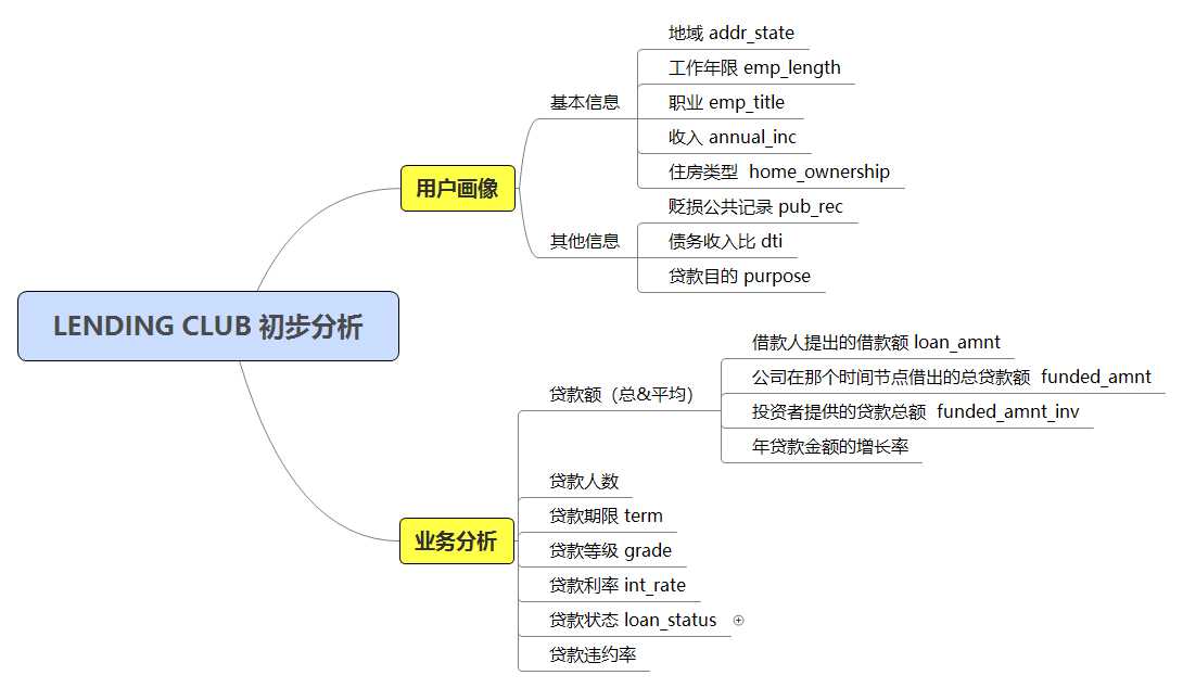
图3 Lending Club 初步分析框架
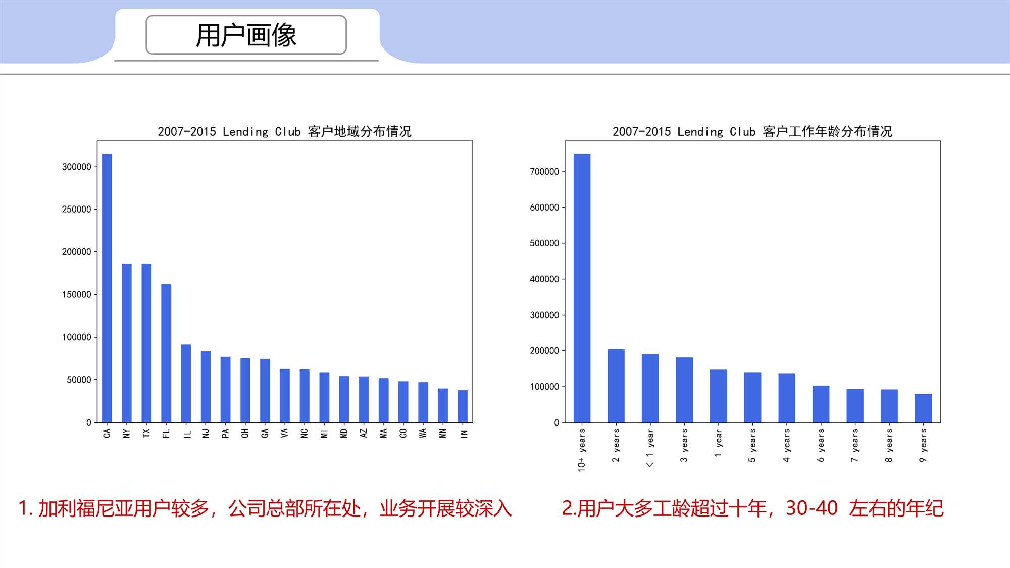
用户画像
加利福尼亚用户较多,公司总部所在处,业务开展较深入
用户大多工龄超过十年,30-40 左右的年纪
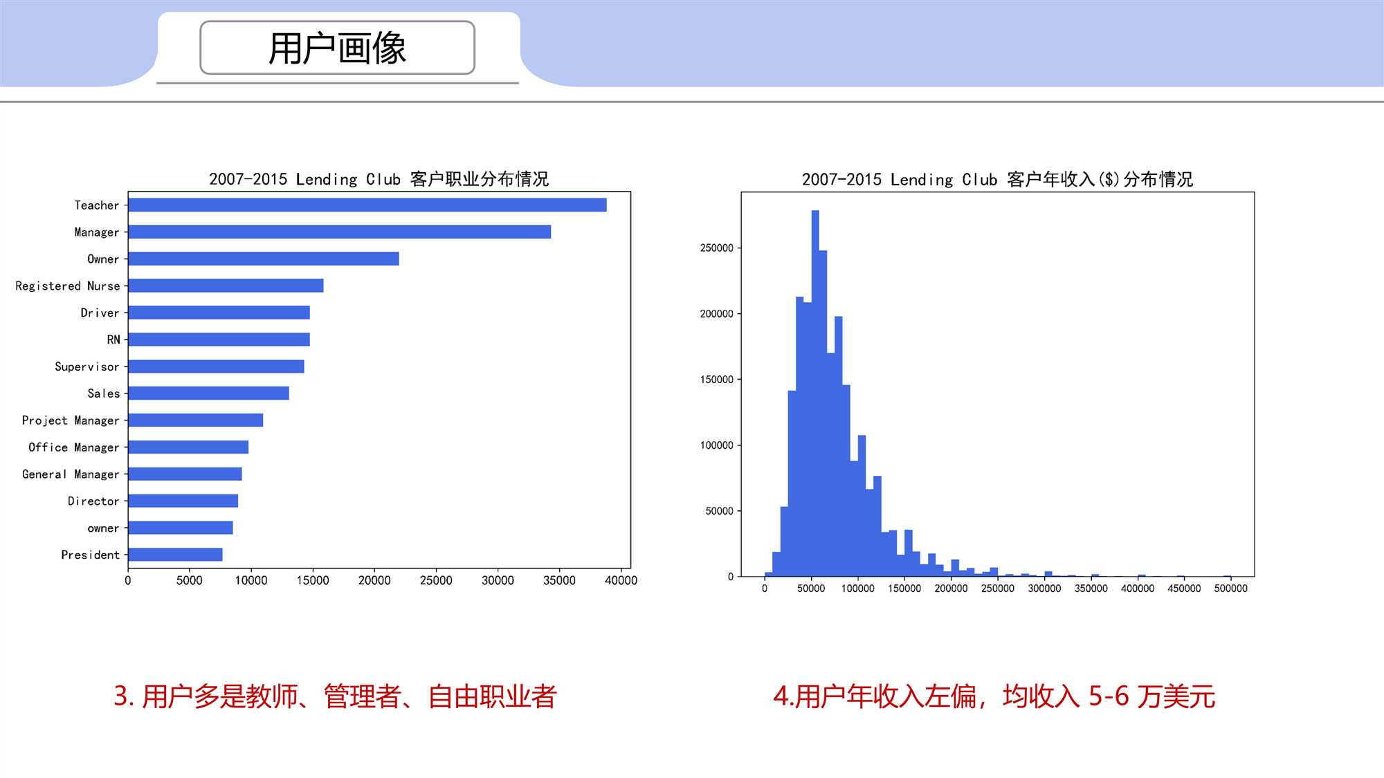
用户多是教师、管理者、自由职业者
用户年收入左偏,均收入 5-6 万美元
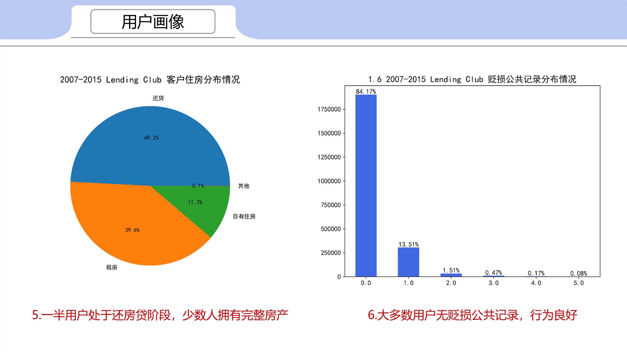
一半用户处于还房贷阶段,少数人拥有完整房产
大多数用户无贬损公共记录,行为良好
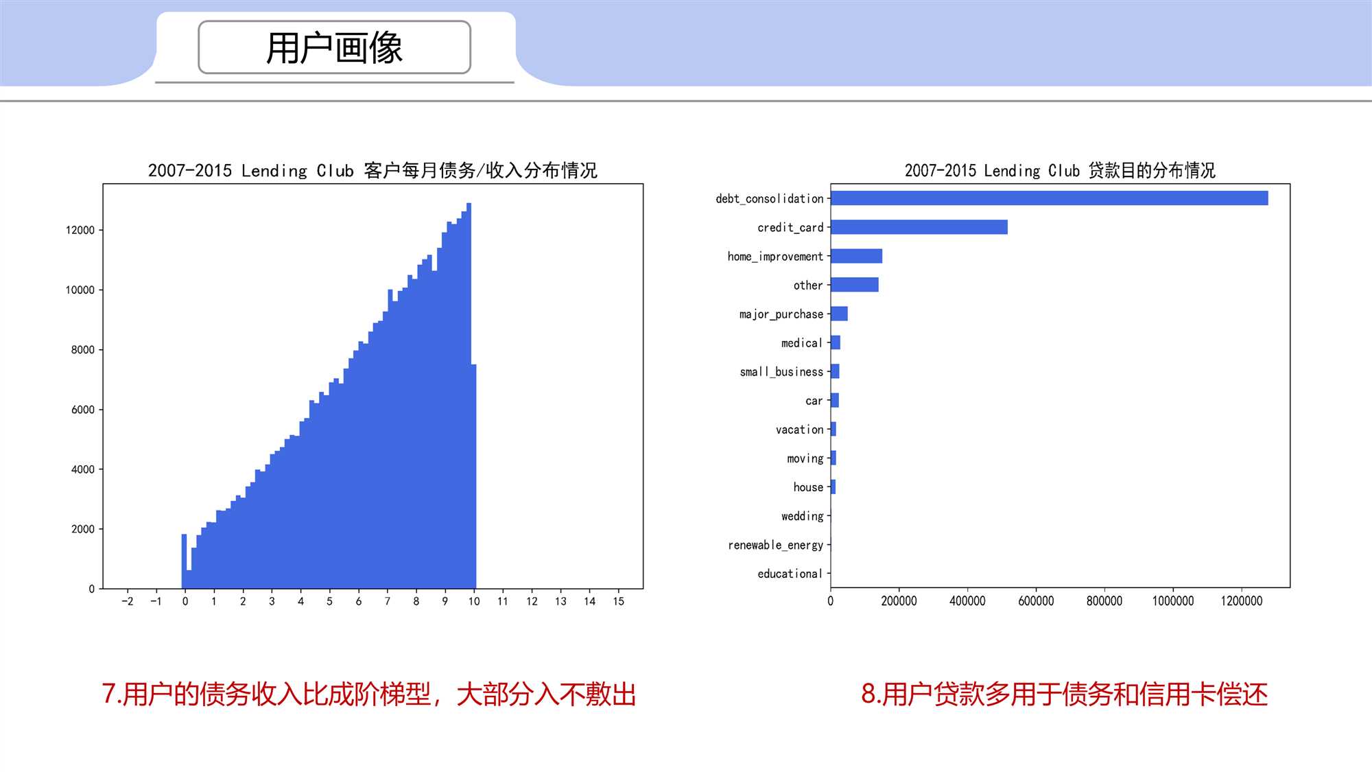
用户的债务收入比成阶梯型,大部分入不敷出
用户贷款多用于债务和信用卡偿还
业务分析
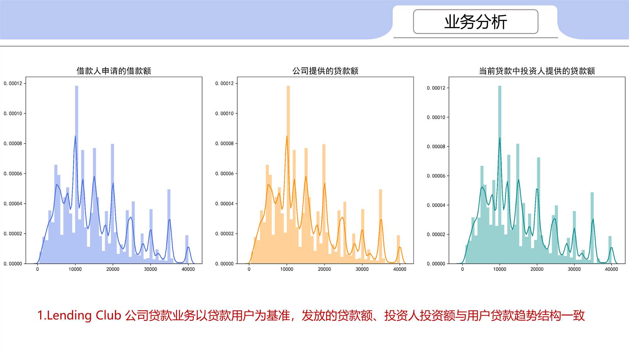
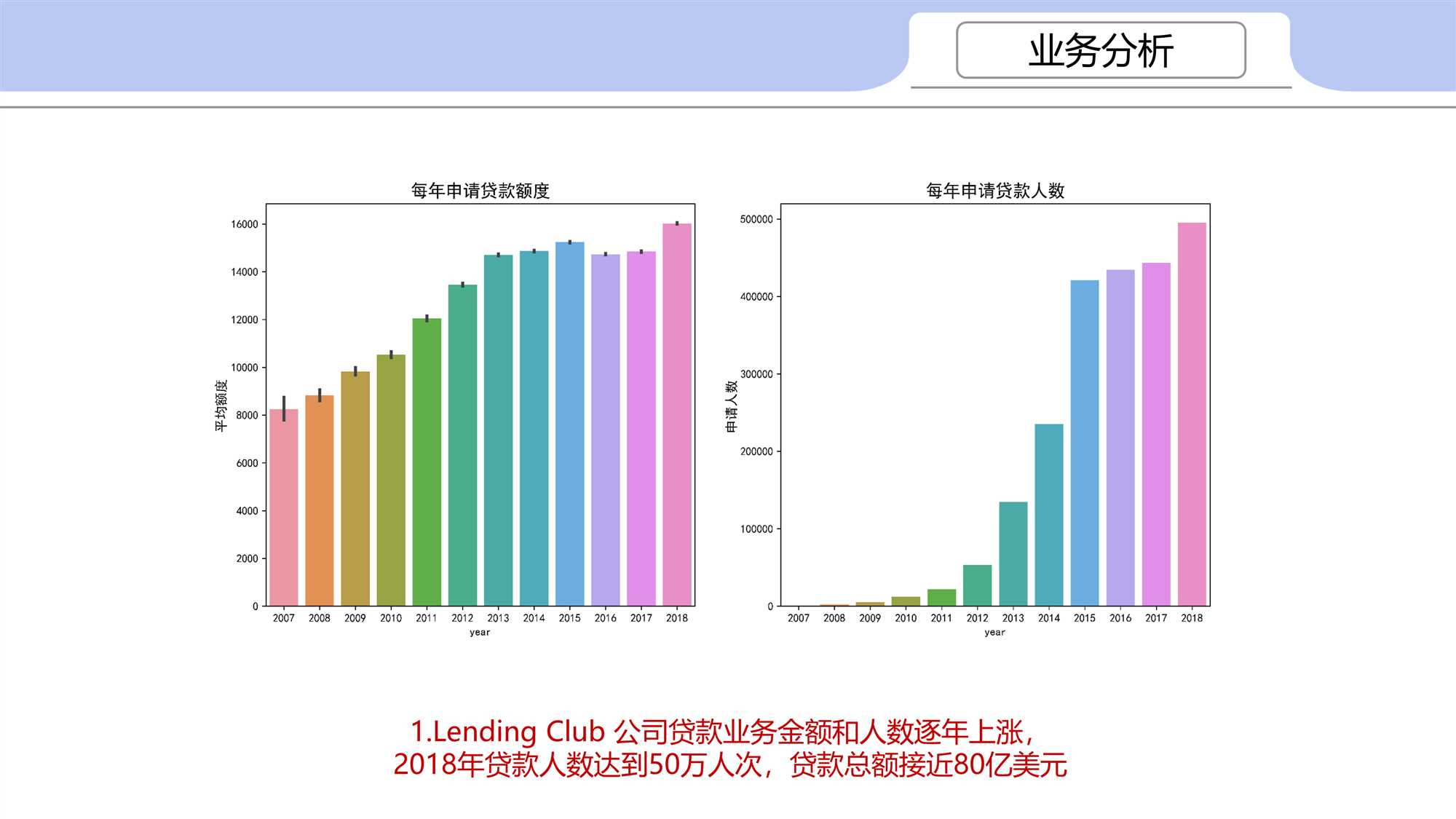
Lending Club 公司贷款业务以贷款用户为基准,发放的贷款额、投资人投资额与用户贷款趋势结构一致
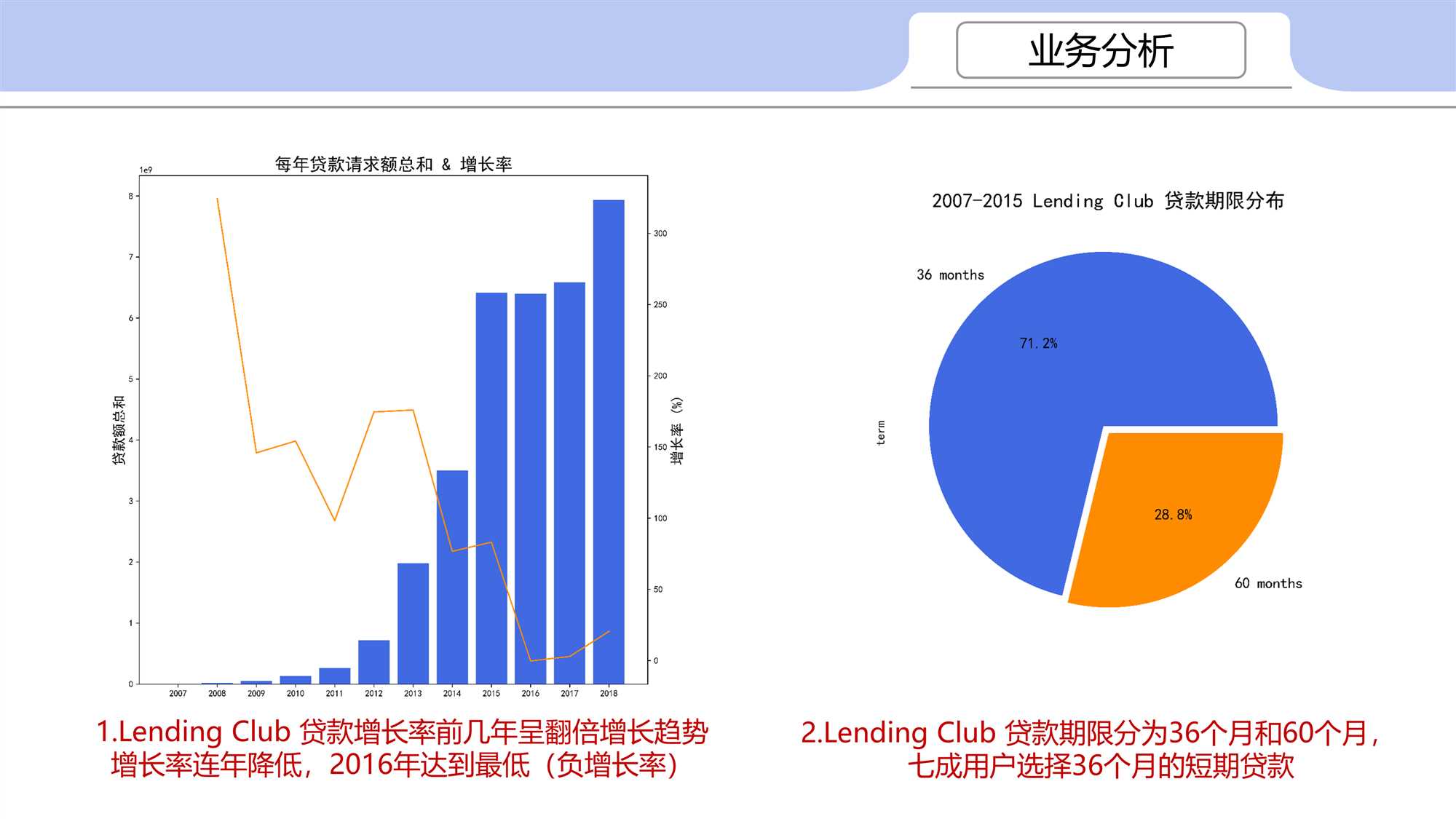
Lending Club 贷款增长率前几年呈翻倍增长趋势,增长率连年降低,2016年达到最低(负增长率,与爆出的丑闻有直接关系)
Lending Club 公司贷款业务金额和人数逐年上涨,
2018年贷款人数达到50万,贷款总额接近80亿美元
Lending Club 贷款期限分为36个月和60个月,七成用户选择36个月的短期贷款
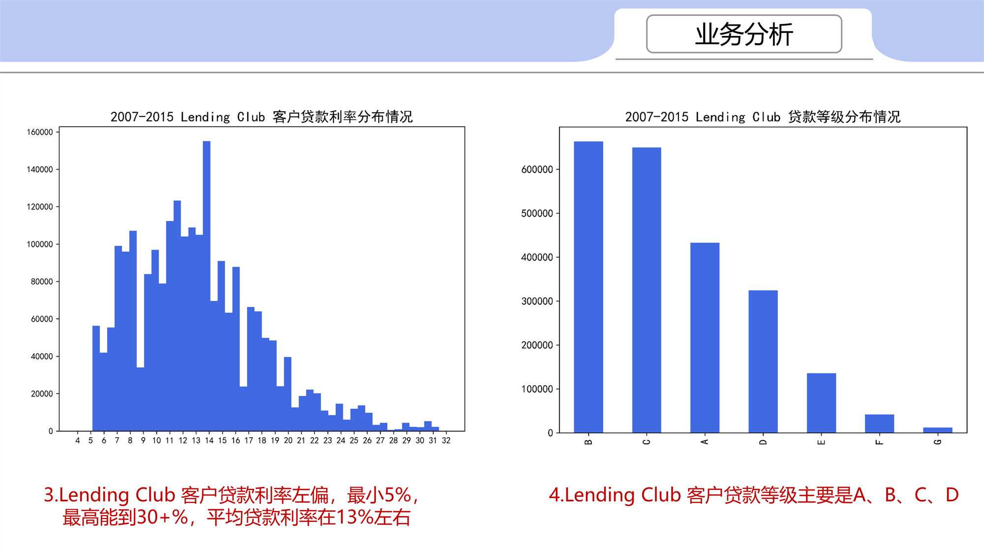
Lending Club 客户贷款利率左偏,最小5%,最高能到30+%,平均贷款利率在13%左右
Lending Club 客户贷款等级主要是A、B、C、D
Lending Club 客户贷款状态良好,绝大多数已付清或者在正常付款中,质量不好的贷款在2015年后逐年下降
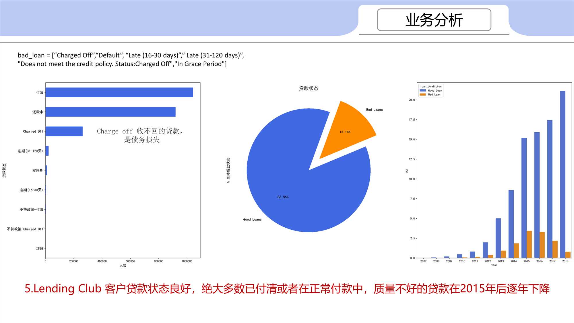
贷款状态说明:
Current 正常还贷中
Fully Paid 付清
Issued 发放
Charged Off 销账,已经收不回来的贷款
Late (31-120 days) 延期
Late (16-30 days) 延期
In Grace Period 宽限期
Does not meet the credit policy. Status:Charged Off 不符合信贷政策,销账
Does not meet the credit policy. Status:Fully Paid 不符合信贷政策,付清
Default 坏账
程序:
#coding:utf-8

import pandas as pd
import numpy as np
import time
import matplotlib.pyplot as plt
import seaborn as sns

plt.rcParams[‘font.sans-serif‘] = [‘SimHei‘]  # 用来正常显示中文标签
plt.rcParams[‘axes.unicode_minus‘] = False    # 用来正常显示负号,#有中文出现的情况,需要u‘内容‘

start_time = time.process_time()

# # 读取数据
# loan = pd.read_csv(‘loan.csv‘,low_memory = False)
# df = loan[[‘issue_d‘,‘addr_state‘,‘emp_length‘, ‘emp_title‘, ‘annual_inc‘,‘home_ownership‘,
#          ‘pub_rec‘, ‘dti‘,‘purpose‘,
#          ‘loan_amnt‘,‘funded_amnt‘,‘funded_amnt_inv‘,‘term‘, ‘grade‘,‘int_rate‘,‘loan_status‘,
#          ‘tot_cur_bal‘,‘avg_cur_bal‘, ‘total_acc‘, ‘total_bc_limit‘,]].copy()
#
# # 将 ‘issue_d’ str形式的时间日期转换
# dt_series = pd.to_datetime(df[‘issue_d‘])
# df[‘year‘] = dt_series.dt.year
# df[‘month‘] = dt_series.dt.month
#
# # 根据收入 ‘annual_inc‘ 定义收入“低、中、高”
# # <10万 --> low , 10万~20万 --> medium , >20 万 --> high
# df[‘income_category‘] = np.nan
# lst = [df]
# for col in lst:
#     col.loc[col[‘annual_inc‘] <= 100000, ‘income_category‘] = ‘Low‘
#     col.loc[(col[‘annual_inc‘] > 100000) & (col[‘annual_inc‘] <= 200000), ‘income_category‘] = ‘Medium‘
#     col.loc[col[‘annual_inc‘] > 200000, ‘income_category‘] = ‘High‘
#
# # 根据贷款状态 ‘loan_status’ 定义好坏贷款
# bad_loan = ["Charged Off",
#             "Default",
#             "Does not meet the credit policy. Status:Charged Off",
#             "In Grace Period",
#             "Late (16-30 days)",
#             "Late (31-120 days)"]
# df[‘loan_condition‘] = np.nan
#
# def loan_condition(status):
#     if status in bad_loan:
#         return ‘Bad Loan‘
#     else:
#         return ‘Good Loan‘
#
# df[‘loan_condition‘] = df[‘loan_status‘].apply(loan_condition)
# df[‘loan_condition_int‘] = np.nan
# for col in lst:
#     col.loc[df[‘loan_condition‘] == ‘Good Loan‘, ‘loan_condition_int‘] = 0  # Negative (Bad Loan)
#     col.loc[df[‘loan_condition‘] == ‘Bad Loan‘, ‘loan_condition_int‘] = 1  # Positive (Good Loan)
# df[‘loan_condition_int‘] = df[‘loan_condition_int‘].astype(int)
#
# df.to_pickle("first_df.pkl")

# 数据查看

df = pd.read_pickle(‘first_df.pkl‘)
# print(df.head())
# print(df.info())
# print(df.describe())
# print(df.isna().sum())          # 检查空值情况


# # 1 客户画像
# # 1.1 地域分布
# fig1 = plt.figure()
# ax1 = fig1.add_subplot(111)
# df[‘addr_state‘].value_counts()[0:19].plot(kind=‘bar‘,color="royalblue",fontsize=12)
# plt.title("2007-2015 Lending Club 客户地域分布情况",fontsize=16)
# plt.subplots_adjust(top=1,bottom=0,left=0,right=1,hspace=0,wspace=0)
# plt.savefig("1.1 2007-2015 Lending Club 客户地域分布情况.png",dpi=1000,bbox_inches = ‘tight‘)#解决图片不清晰,不完整的问题
# # plt.show()
#
# # 1.2 工作年限分布
# fig2 = plt.figure()
# ax1 = fig2.add_subplot(111)
# df[‘emp_length‘].value_counts().plot(kind=‘bar‘,color="royalblue",fontsize=12)
# plt.title("2007-2015 Lending Club 客户工作年龄分布情况",fontsize=16)
# plt.subplots_adjust(top=1,bottom=0,left=0,right=1,hspace=0,wspace=0)
# plt.savefig("1.2 2007-2015 Lending Club 客户工作年龄分布情况.png",dpi=1000,bbox_inches = ‘tight‘)#解决图片不清晰,不完整的问题
# # plt.show()
#
# # 1.3 职业分布
# fig3 = plt.figure()
# ax1 = fig3.add_subplot(111)
# df[‘emp_title‘].value_counts()[0:14][::-1].plot(kind=‘barh‘,color="royalblue",fontsize=12)
# plt.title("2007-2015 Lending Club 客户职业分布情况",fontsize=16)
# plt.subplots_adjust(top=1,bottom=0,left=0,right=1,hspace=0,wspace=0)
# plt.savefig("1.3 2007-2015 Lending Club 客户职业分布情况.png",dpi=1000,bbox_inches = ‘tight‘)#解决图片不清晰,不完整的问题
# # plt.show()
#
# # 1.4 收入分布
# fig4 = plt.figure()
# ax1 = fig4.add_subplot(111)
# new_ticks=np.linspace(0,500000,11)
# plt.hist(df[‘annual_inc‘].dropna(),range=(0,500000),bins=60,color="royalblue")
# plt.xticks(new_ticks)
# plt.title("2007-2015 Lending Club 客户年收入($)分布情况",fontsize=16)
# plt.subplots_adjust(top=1,bottom=0,left=0,right=1,hspace=0,wspace=0)
# plt.savefig("1.4 2007-2015 Lending Club 客户年收入($)分布情况.png",dpi=1000,bbox_inches = ‘tight‘) # 解决图片不清晰,不完整的问题
# # plt.show()
#
# # 1.5 住房类型分布
# fig5 = plt.figure()
# ax1 = fig5.add_subplot(111)
# df[‘home_ownership‘].replace({"MORTGAGE":"还贷","RENT":"租房","OWN":"自有住房","ANY":"其他","OTHER":"其他","NONE":"其他"},inplace=True)
# plt.pie(df[‘home_ownership‘].dropna().value_counts(),labels=["还贷","租房","自有住房","其他"],autopct="%1.1f%%")
# plt.title("2007-2015 Lending Club 客户住房分布情况",fontsize=16)
# plt.subplots_adjust(top=1,bottom=0,left=0,right=1,hspace=0,wspace=0)
# plt.savefig("1.5 2007-2015 Lending Club 客户住房分布情况.png",dpi=1000,bbox_inches = ‘tight‘) # 解决图片不清晰,不完整的问题
# # plt.show()
#
# # 1.6 贬损公共记录
# fig6 = plt.figure()
# ax1 = fig6.add_subplot(111)
# pub_v=df[‘pub_rec‘].value_counts()
# x_ticks=list(range(6))
# pub_v[0:5].plot(kind=‘bar‘,color=‘royalblue‘,fontsize=12)
# plt.xticks(x_ticks,rotation=0)
# pub_p=pub_v/pub_v.sum()     # 计算所占百分比
# pub_p=pub_p.apply(lambda x:format(x,‘.2%‘))[0:5] # 转换百分比显示
# for i in x_ticks:
#     plt.text(i,pub_v[i]+1.2, pub_p[i], ha=‘center‘, va= ‘bottom‘,fontsize=12)
# plt.title("1.6 2007-2015 Lending Club 贬损公共记录分布情况",fontsize=16)
# plt.subplots_adjust(top=1,bottom=0,left=0,right=1,hspace=0,wspace=0)
# plt.savefig("1.6 2007-2015 Lending Club 贬损公共记录分布情况.png",dpi=1000,bbox_inches = ‘tight‘) # 解决图片不清晰,不完整的问题
# # plt.show()
#
# # 1.7 债务收入比
# fig7=plt.figure()
# ax1=fig7.add_subplot(111)
# new_ticks=np.linspace(-2,15,18)
# plt.hist(df[‘dti‘][df[‘dti‘]<10].dropna(),range=(-2,15),bins=100,color="royalblue")
# plt.xticks(new_ticks)
# plt.title("2007-2015 Lending Club 客户每月债务/收入分布情况",fontsize=16)
# plt.subplots_adjust(top=1,bottom=0,left=0,right=1,hspace=0,wspace=0)
# plt.savefig("1.7 2007-2015 Lending Club 客户每月 债务-收入比分布情况.png",dpi=1000,bbox_inches = ‘tight‘)#解决图片不清晰,不完整的问题
# # plt.show()
#
#
# # 1.8 贷款目的
# fig8 = plt.figure()
# ax1 = fig8.add_subplot(111)
# df[‘purpose‘].value_counts(ascending=True).plot(kind=‘barh‘,fontsize=12,color="royalblue")
# plt.title("2007-2015 Lending Club 贷款目的分布情况",fontsize=16)
# plt.subplots_adjust(top=1,bottom=0,left=0,right=1,hspace=0,wspace=0)
# plt.savefig("1.8 2007-2015 Lending Club 贷款目的分布情况.png",dpi=1000,bbox_inches = ‘tight‘)#解决图片不清晰,不完整的问题
# plt.show()

#
#
# # 2 业务分析
# # 2.1 贷款额(总&平均)
# fig1, ax = plt.subplots(1, 3, figsize=(16,5))
# loan_amount = df["loan_amnt"].values
# funded_amount = df["funded_amnt"].values
# investor_funds = df["funded_amnt_inv"].values
#
# sns.distplot(loan_amount, ax=ax[0], color="royalblue")
# ax[0].set_title("借款人申请的借款额", fontsize=16)
# sns.distplot(funded_amount, ax=ax[1], color="darkorange")
# ax[1].set_title("公司提供的贷款额", fontsize=16)
# sns.distplot(investor_funds, ax=ax[2], color="darkcyan")
# ax[2].set_title("当前贷款中投资人提供的贷款额", fontsize=16)
# plt.subplots_adjust(top=1,bottom=0,left=0,right=1,hspace=0.2,wspace=0.2)
# plt.savefig("2.1 2007-2015 Lending Club 贷款情况了解.png",dpi=1000,bbox_inches = ‘tight‘)#解决图片不清晰,不完整的问题
# # plt.show()

# # 每年贷款增长率
# df_g = df[[‘year‘,‘loan_amnt‘]].groupby([‘year‘]).sum().reset_index()
# df_g = df_g.rename(columns={‘loan_amnt‘:‘loan_amnt_sum‘})
# df_g[‘loan_amnt_pro‘] = -df_g[‘loan_amnt_sum‘].diff(-1)/df_g.iloc[:,1]*100
#
# fig11 = plt.figure(figsize=(8,8))
# plt.title("每年贷款请求额总和 & 增长率",fontsize=20)
# plt.bar(df_g.iloc[:,0],df_g.iloc[:,1],color="royalblue")
# plt.ylabel("贷款额总和",fontsize=16)
# plt.xticks(df_g.iloc[:,0])
# plt.twinx()
# plt.plot(df_g.iloc[1:,0],df_g.iloc[:-1,2],color="darkorange")
# plt.ylabel("增长率 (%)",fontsize=16)
# plt.subplots_adjust(top=1,bottom=0,left=0,right=1,hspace=0.2,wspace=0.2)
# plt.savefig("2.11 2007-2015 Lending Club 每年贷款请求额总和&增长率.png",dpi=1000,bbox_inches = ‘tight‘)#解决图片不清晰,不完整的问题
# # plt.show()

# # 2.2 贷款人数
# fig2,ax=plt.subplots(1,2,figsize=(12,5))
# sns.barplot(‘year‘, ‘loan_amnt‘, data=df[[‘year‘,‘loan_amnt‘]],ax=ax[0])
# ax[0].set_title(‘每年申请贷款额度‘, fontsize=16)
# ax[0].set_ylabel("平均额度",fontsize=12)
# sns.countplot(‘year‘,data=df[[‘year‘,‘loan_amnt‘]],ax=ax[1])
# ax[1].set_title(‘每年申请贷款人数‘, fontsize=16)
# ax[1].set_ylabel("申请人数",fontsize=12)
# plt.subplots_adjust(top=1,bottom=0,left=0,right=1,hspace=0.2,wspace=0.2)
# plt.savefig("2.2 2007-2015 Lending Club 每年申请贷款平均额和申请贷款人数.png",dpi=1000,bbox_inches = ‘tight‘)#解决图片不清晰,不完整的问题
# # plt.show()
#
#
# # 2.3 贷款期限
# fig3 = plt.figure()
# colors = [‘royalblue‘,‘darkorange‘]
# df[‘term‘].value_counts().plot(kind=‘pie‘,explode=(0.05,0),autopct="%1.1f%%",colors=colors,fontsize=12)
# plt.title("2007-2015 Lending Club 贷款期限分布",fontsize=16)
# plt.subplots_adjust(top=1,bottom=0,left=0,right=1,hspace=0.2,wspace=0.2)
# plt.savefig("2.3 2007-2015 Lending Club 贷款期限分布.png",dpi=1000,bbox_inches = ‘tight‘)#解决图片不清晰,不完整的问题
# # plt.show()
#
# # 2.4 贷款等级 grade
# fig4 = plt.figure()
# ax1 = fig4.add_subplot(111)
# df[‘grade‘].value_counts().plot(kind=‘bar‘,color="royalblue",fontsize=12)
# plt.title("2007-2015 Lending Club 贷款等级分布情况",fontsize=16)
# plt.subplots_adjust(top=1,bottom=0,left=0,right=1,hspace=0,wspace=0)
# plt.savefig("2.4 2007-2015 Lending Club 贷款等级分布分布情况.png",dpi=1000,bbox_inches = ‘tight‘)#解决图片不清晰,不完整的问题
# # plt.show()
#
# # 2.5 贷款利率 int_rate
# fig5 = plt.figure()
# ax1 = fig5.add_subplot(111)
# new_ticks=np.linspace(4,32,29)
# plt.hist(df[‘int_rate‘],range=(4,32),bins=50,color="royalblue")
# plt.xticks(new_ticks)
# plt.title("2007-2015 Lending Club 客户贷款利率分布情况",fontsize=16)
# plt.subplots_adjust(top=1,bottom=0,left=0,right=1,hspace=0,wspace=0)
# plt.savefig("2.5 2007-2015 Lending Club 客户贷款利率分布情况.png",dpi=1000,bbox_inches = ‘tight‘)#解决图片不清晰,不完整的问题
# # plt.show()
#
#
# # 2.6 贷款状态 loan_status
# fig6, ax = plt.subplots(1,3, figsize=(24,8))
# colors = ["royalblue", "darkorange"]
# statu_labels = [‘付清‘ ,‘还款中‘ ,‘Charged Off‘,
#                 ‘逾期(31-120天)‘ ,‘宽限期‘ ,‘逾期(16-30天)‘ ,
#                 ‘不符政策-付清‘,‘不符政策-Charged Off‘,‘坏账‘]
# labels =["Good Loans", "Bad Loans"]
# print(df[‘loan_status‘].unique())
# plt.suptitle(‘贷款状态‘, fontsize=16)
#
# df["loan_status"].value_counts()[::-1].plot(kind=‘barh‘,color=‘royalblue‘,ax=ax[0])
# ax[0].set_xlabel(‘人数‘,fontsize=12)
# ax[0].set_ylabel(‘贷款状态‘,fontsize=12)
# ax[0].set_yticklabels(statu_labels[::-1
#                       ],fontsize=12)
#
# df["loan_condition"].value_counts().plot.pie(explode=[0,0.25], autopct=‘%1.2f%%‘, ax=ax[1], shadow=False, colors=colors,
#                                              labels=labels, fontsize=12, startangle=70)
# ax[1].set_ylabel(‘% 总体贷款状态‘, fontsize=12)
#
# sns.barplot(x="year", y="loan_amnt", hue="loan_condition", data=df, palette=colors,ax=ax[2], estimator=lambda x: len(x) / len(df[‘year‘]) * 100)
# ax[2].set(ylabel="(%)")
# plt.subplots_adjust(top=1,bottom=0,left=0,right=1,hspace=0.2,wspace=0.2)
# plt.savefig("2.6 2007-2015 Lending Club 贷款状态分布.png",dpi=1000,bbox_inches = ‘tight‘) #解决图片不清晰,不完整的问题
# # plt.show()


end_time = time.process_time()
print("程序运行了 %s 秒"%(end_time-start_time))
Lending Club 公司2007-2018贷款业务初步分析
标签:xpl lock ddr unicode 大型 直接 val 快速 读取
原文地址:https://www.cnblogs.com/Ray-0808/p/12618551.html