标签:first camera distance def comment rman mos bec axis
Week 2 3.5.2020
This week, we have mainly learned two parts:
1. How to match the same feature points in two images from different viewpoints.
2. The mathematic model of the pinhole camera.
To reconstruct a 3-D object, the basic processes can be divided into 2 steps. The first is to obtain some feature points in two or more images from different viewpoints by using e.g. Harris corner detector. The second step is to match the corresponding feature points from the images. Mathematically, \(V_i\) and [W_i\) donate the feature points in two images, respectively. We want to find the \(V_i\) and \(W_j\) which represent the same feature points. But the second image always contains the rotated and scaled version of the feature points in the first image because of the different viewpoints and different situations of cameras. If we just find the smallest distance of two feature points, we maybe get the wrong matching. The rotation and intensity compensations should be considered.
The angle of a feature point is defined as \( \theta = arctan( \frac{\frac{\partial I}{\partial x_2} }{\frac{\partial I}{\partial x_1}}) \) where \(x_2\) donates the horizontal axis and \(x_1\) donates the vertical axis. Rotate the \(theta\) so that the orientations of the two features should be equal.
The difference in intensities also leads to mismatching of feature points. in another words, the feature points are sensitive to the illumination. The intensities of two matched feature points should be almost equal. \( W \approx \alpha V + \beta \mathbb{1} \mathbb{1}^T \) \( \alpha \) represents the scalar of intensities and \(beta\)\ represents the bias.
\( \mathbb{1} \mathbb{1}^T= \begin{matrix} 1 & 1& \cdots &1 \\ 1 & 1& \cdots & 1 \\ \vdots & \vdots & \ddots & \vdots \\ 1& 1& \cdots & 1 \end{matrix} \)
Normalization of the feature points to remove the effects of different intensities.
\( W_n = \frac{1}{ \sigma(W)} (W-\overline{W}) \)
mean value is
\( \begin{aligned} \bar{W} &=\frac{1}{N}\left(\mathbb{1} \mathbb{1}^{\top} W \mathbb{1} \mathbb{T}\right) \& \approx \frac{1}{N}\left(\mathbb{1} \mathbb{1}^{\top}\left(\alpha V+\beta \mathbb{1}^{\top}\right) \mathbb{1} \mathbb{1}^{\top}\right) \&=\alpha \frac{1}{N}\left(\mathbb{1} \mathbb{1}^{\top} V \mathbb{1} \mathbb{1}^{\top}\right)+\beta \mathbb{1}^{\top} \&=\alpha \bar{V}+\beta \mathbb{1}^{\top} \end{aligned} \)
variance is
\( \begin{aligned} \sigma(W) &=\sqrt{\frac{1}{N-1}\|W-\bar{W}\|_{F}^{2}} \&=\sqrt{\frac{1}{N-1} \operatorname{tr}\left((W-\bar{W})^{\top}(W-\bar{W})\right)} \& \approx \sqrt{\frac{1}{N-1} \operatorname{tr}\left(\alpha(V-\bar{V})^{\top} \alpha(V-\bar{V})\right)} \&=\alpha \sigma(V) \end{aligned} \)
By using SSD or NCC we can calculate the distance of different normalized feature points.
SSD :
\( d(V,W) = ||V-W||^2_F =2(N-1)-2tr(W_n^TV_n) \)
\( ||A||^2_F = tr(A^TA) = \sum_{ij} a_{ij}^2 \)
NCC:
\( \frac{1}{N-1}{tr(W_n^TV_n)} \)
Comment
NCC and SSD are very fast algorithms for block matching. They have outstanding performances in normal situations because the intensity and rotation information have been compensated and they are fast enough to deal with hundreds of feature blocks. But in practice, the feature points always have different scalar information as in Figure 1. It is hard to apply the NCC algorithm to match traffic light. In this scenario, the SSD or NCC is sensitive to scalar information.

Figure 1 feature points with different scalar information
In modern feature matching algorithms, a common way is to build a unique descriptor for every feature. The descriptor should be:
1. Scalar and rotation invariant. The descriptor should be calculated without the influence of scalar and rotation information.
2. Robust. The descriptor can not be sensitive to illumination and noise information.
3. Unique descriptor. The descriptor should be distinguishable for different feature points.
NCC satisfies the last two requirements by intensities and rotation compensation. To achieve the scalar invariant, a common way is to build a scalar pyramid. Figure 2 shows how a gauss pyramid is built. every level of the pyramid is the subsampling of the last level. According to the hierarchy, the different scalar information of the feature points have been shown.

Figure 2 scalar pyramid
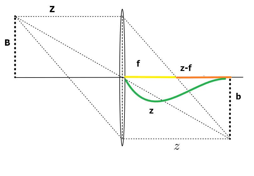
the basic principle of the camera is the Pinhole model which can project a 3D object to a 2D flat by using a lens. Figure 3 shows a simple model of a pinhole camera.

Figure3 pinhole model
\( \left|\frac{b}{B}\right|=\frac{z-f}{f}\\left|\frac{z}{Z}\right|=\left|\frac{b}{B}\right|\\Rightarrow \frac{z}{f}-1 = \frac{z}{|Z|}\\Rightarrow \frac{1}{f}-\frac{1}{z} = \frac{1}{|Z|}\\Rightarrow \frac{1}{|Z|} +\frac{1}{z}=\frac{1}{f} \)
As a result the length of object is proportional to the mirrored image.
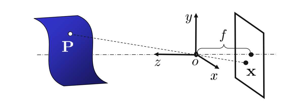
In the pinhole model, every point in the 3-D space will be projected into 2-D. We can see the relationship between the 3-D object and 2-D images in Figure 4.

Figure 4 projection relationship
If the original point in the 3-D space is\( (X,Y,Z) \), the point will be projected into \( (-\frac{fX}{Z},-\frac{fY}{Z},-f) \) . The Z-axis is constant, we can say that a dimension has been canceled, and the coordinates in X and Y directions in the image are related to f and Z. If we take the image in front of the lens, we can get (\frac{fX}{Z},\frac{Y}{Z},f).
标签:first camera distance def comment rman mos bec axis
原文地址:https://www.cnblogs.com/deuchen/p/12872725.html