标签:state ext import eric osi drop spl 准备 防止
数据准备是机器学习中一项非常重要的环节,本文主要对数据准备流程进行简单的梳理,主要参考了Data Preparation for Machine Learning一书。
数据准备需要进行的工作主要分为以下几类:
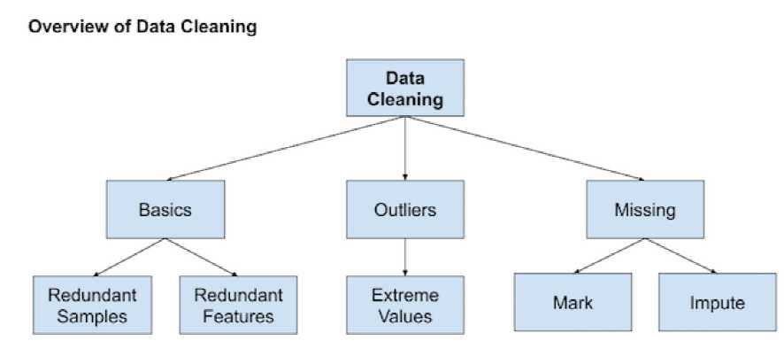
# delete columns with a single unique value
counts = df.nunique()
to_del = [i for i,v in enumerate(counts) if v == 1]
df.drop(to_del, axis=1, inplace=True)

# delete rows of duplicate data from the dataset
df.drop_duplicates(inplace=True)
# identify outliers in the training dataset
lof = LocalOutlierFactor()
yhat = lof.fit_predict(X_train)
# Method 1: select all rows that are not outliers
mask = yhat != -1
X_train, y_train = X_train[mask, :], y_train[mask]
# Method 2: check LOF score
score = lof.negative_outlier_factor_
X_train, y_train = X_train[score>threshold], y_train[score>threshold]
rng = np.random.RandomState(42)
clf = IsolationForest(max_samples=256,  random_state=rng, contamination=‘auto‘)
yhat = clf.fit_predict(X_train)
mask = yhat != -1
X_train, y_train = X_train[mask, :], y_train[mask]
# define imputer
imputer = SimpleImputer(strategy=‘mean‘)
# fit on the training dataset (fit函数仅在训练数据上使用,防止data leakage)
Xtrans = imputer.fit_transform(X_train)
pipeline = Pipeline(steps=[(‘i‘, KNNImputer(n_neighbors=...)), (‘m‘, RandomForestClassifier())])
# evaluate the model
cv = RepeatedStratifiedKFold(n_splits=10, n_repeats=3, random_state=1)
scores = cross_val_score(pipeline, X, y, scoring=‘accuracy‘, cv=cv, n_jobs=-1)
##############################################################
#1. 对每个缺失值进行初始填充
#2. 根据选定的特征顺序依次对有缺失值的特征建立预测模型,将其表示为其它特征的函数,训练模型并预测该特征的缺失值,使用预测值更新缺失值
#3. 不断重复上一步骤进行迭代
##############################################################

# estimator: 使用的预测模型
# imputation_order: 进行缺失值更新和填充的特征顺序
# n_nearest_features: 模型训练和预测使用的特征数量
# max_iter: 最大迭代次数
# initial_strategy: 初始填充使用的填充策略
pipeline = Pipeline(steps=[(‘i‘, IterativeImputer(estimator=..., max_iter=..., n_nearest_features=..., initial_strategy=..., imputation_order=...)), (‘m‘, RandomForestClassifier())])
# evaluate the model
cv = RepeatedStratifiedKFold(n_splits=10, n_repeats=3, random_state=1)
scores = cross_val_score(pipeline, X, y, scoring=‘accuracy‘, cv=cv, n_jobs=-1)
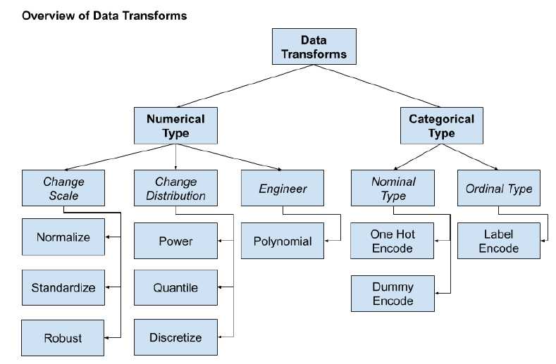
# prepare the model with input scaling and power transform
steps = list()
steps.append((‘scale‘, MinMaxScaler(feature_range=(1e-5,1))))
steps.append((‘power‘, PowerTransformer()))
steps.append((‘model‘, HuberRegressor()))
pipeline = Pipeline(steps=steps)
# prepare the model with target power transform
model = TransformedTargetRegressor(regressor=pipeline, transformer=PowerTransformer())
# evaluate model
cv = RepeatedKFold(n_splits=10, n_repeats=3, random_state=1)
scores = cross_val_score(model, X, y, scoring=‘neg_mean_absolute_error‘, cv=cv, n_jobs=-1)
# determine categorical and numerical features
numerical_ix = X.select_dtypes(include=[‘int64‘, ‘float64‘]).columns
categorical_ix = X.select_dtypes(include=[‘object‘, ‘bool‘]).columns
# define the data preparation for the columns
t = [(‘cat‘, OneHotEncoder(), categorical_ix), (‘num‘, MinMaxScaler(), numerical_ix)]
col_transform = ColumnTransformer(transformers=t, remainder=...)
# define the data preparation and modeling pipeline
pipeline = Pipeline(steps=[(‘prep‘,col_transform), (‘m‘, model)])
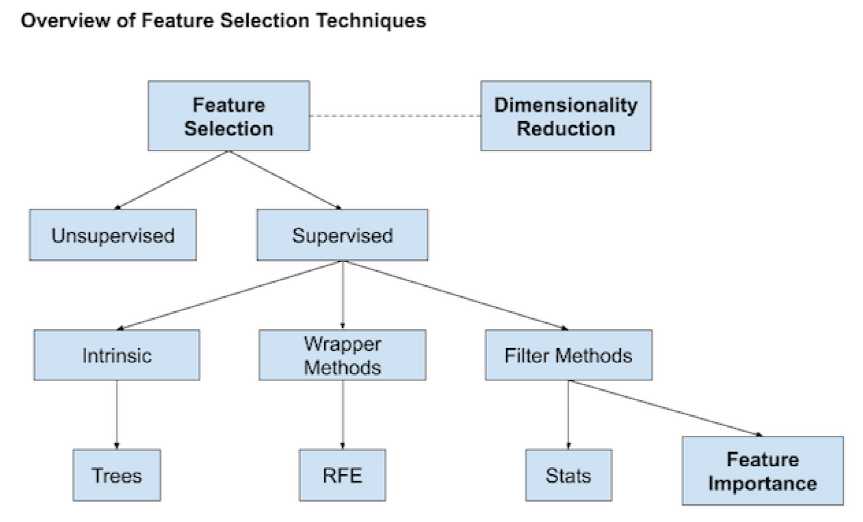
SelectKBest(score_func=chi2, k=...)
SelectKBest(score_func=mutual_info_classif, k=...)  #classification
SelectKBest(score_func=mutual_info_regression, k=...)  #regression
SelectKBest(score_func=f_classif, k=...)
SelectKBest(score_func=f_regression, k=...)
SelectFromModel(estimator=..., max_features=..., threshold=...)
SelectFromModel(estimator=..., max_features=..., threshold=...)
### Example 1 ###
model = KNeighborsRegressor()
model.fit(X_train, y_train) # fit the model
# perform permutation importance
results = permutation_importance(model, X_train, y_train, scoring=‘neg_mean_squared_error‘)
importance = results.importances_mean  #get importance

### Example 2 ###
model = Ridge(alpha=1e-2).fit(X_train, y_train)
r = permutation_importance(model, X_val, y_val, n_repeats=30, random_state=0)
importance = r.importances_mean
RFE(estimator=..., n_features_to_select=..., step=...)
Dimension Reduction: LDA(有监督降维), PCA(无监督降维),算法原理可参考PCA与LDA介绍
标签:state ext import eric osi drop spl 准备 防止
原文地址:https://www.cnblogs.com/sunwq06/p/11346738.html