标签:axis fse 方式 oss conv2 选项 scale 场景 对比
S. K. Roy, G. Krishna, S. R. Dubey, B. B. Chaudhuri HybridSN: Exploring 3-D–2-D CNN Feature Hierarchy for Hyperspectral Image Classification, IEEE GRSL 2020
这篇论文构建了一个 混合网络 解决高光谱图像分类问题,首先用 3D卷积,然后使用 2D卷积,代码相对简单,下面是代码的解析。
首先取得数据,并引入基本函数库。
! wget http://www.ehu.eus/ccwintco/uploads/6/67/Indian_pines_corrected.mat
! wget http://www.ehu.eus/ccwintco/uploads/c/c4/Indian_pines_gt.mat
! pip install spectral
import numpy as np
import matplotlib.pyplot as plt
import scipy.io as sio
from sklearn.decomposition import PCA
from sklearn.model_selection import train_test_split
from sklearn.metrics import confusion_matrix, accuracy_score, classification_report, cohen_kappa_score
import spectral
import torch
import torchvision
import torch.nn as nn
import torch.nn.functional as F
import torch.optim as optim
模型的网络结构为如下图所示:
下面是 HybridSN 类的代码:
class_num = 16
class HybridSN(nn.Module):
  def __init__(self):
    super(HybridSN, self).__init__()
    self.conv3d_1 = nn.Sequential(
        nn.Conv3d(1, 8, kernel_size=(7, 3, 3), stride=1, padding=0),
        nn.BatchNorm3d(8),
        nn.ReLU(inplace = True),
    )
    self.conv3d_2 = nn.Sequential(
        nn.Conv3d(8, 16, kernel_size=(5, 3, 3), stride=1, padding=0),
        nn.BatchNorm3d(16),
        nn.ReLU(inplace = True),
    )
    self.conv3d_3 = nn.Sequential(
        nn.Conv3d(16, 32, kernel_size=(3, 3, 3), stride=1, padding=0),
        nn.BatchNorm3d(32),
        nn.ReLU(inplace = True)
    )

    self.conv2d_4 = nn.Sequential(
        nn.Conv2d(576, 64, kernel_size=(3, 3), stride=1, padding=0),
        nn.BatchNorm2d(64),
        nn.ReLU(inplace = True),
    )
    self.fc1 = nn.Linear(18496,256)
    self.fc2 = nn.Linear(256,128)
    self.fc3 = nn.Linear(128,16)
    self.dropout = nn.Dropout(p = 0.4)

  def forward(self,x):
    out = self.conv3d_1(x)
    out = self.conv3d_2(out)
    out = self.conv3d_3(out)
    out = self.conv2d_4(out.reshape(out.shape[0],-1,19,19))
    out = out.reshape(out.shape[0],-1)
    out = F.relu(self.dropout(self.fc1(out)))
    out = F.relu(self.dropout(self.fc2(out)))
    out = self.fc3(out)
    return out
# 对高光谱数据 X 应用 PCA 变换
def applyPCA(X, numComponents):
    newX = np.reshape(X, (-1, X.shape[2]))
    pca = PCA(n_components=numComponents, whiten=True)
    newX = pca.fit_transform(newX)
    newX = np.reshape(newX, (X.shape[0], X.shape[1], numComponents))
    return newX

# 对单个像素周围提取 patch 时,边缘像素就无法取了,因此,给这部分像素进行 padding 操作
def padWithZeros(X, margin=2):
    newX = np.zeros((X.shape[0] + 2 * margin, X.shape[1] + 2* margin, X.shape[2]))
    x_offset = margin
    y_offset = margin
    newX[x_offset:X.shape[0] + x_offset, y_offset:X.shape[1] + y_offset, :] = X
    return newX

# 在每个像素周围提取 patch ,然后创建成符合 keras 处理的格式
def createImageCubes(X, y, windowSize=5, removeZeroLabels = True):
    # 给 X 做 padding
    margin = int((windowSize - 1) / 2)
    zeroPaddedX = padWithZeros(X, margin=margin)
    # split patches
    patchesData = np.zeros((X.shape[0] * X.shape[1], windowSize, windowSize, X.shape[2]))
    patchesLabels = np.zeros((X.shape[0] * X.shape[1]))
    patchIndex = 0
    for r in range(margin, zeroPaddedX.shape[0] - margin):
        for c in range(margin, zeroPaddedX.shape[1] - margin):
            patch = zeroPaddedX[r - margin:r + margin + 1, c - margin:c + margin + 1]
            patchesData[patchIndex, :, :, :] = patch
            patchesLabels[patchIndex] = y[r-margin, c-margin]
            patchIndex = patchIndex + 1
    if removeZeroLabels:
        patchesData = patchesData[patchesLabels>0,:,:,:]
        patchesLabels = patchesLabels[patchesLabels>0]
        patchesLabels -= 1
    return patchesData, patchesLabels

def splitTrainTestSet(X, y, testRatio, randomState=345):
    X_train, X_test, y_train, y_test = train_test_split(X, y, test_size=testRatio, random_state=randomState, stratify=y)
    return X_train, X_test, y_train, y_test
# 地物类别
class_num = 16
X = sio.loadmat(‘Indian_pines_corrected.mat‘)[‘indian_pines_corrected‘]
y = sio.loadmat(‘Indian_pines_gt.mat‘)[‘indian_pines_gt‘]

# 用于测试样本的比例
test_ratio = 0.90
# 每个像素周围提取 patch 的尺寸
patch_size = 25
# 使用 PCA 降维,得到主成分的数量
pca_components = 30

print(‘Hyperspectral data shape: ‘, X.shape)
print(‘Label shape: ‘, y.shape)

print(‘\n... ... PCA tranformation ... ...‘)
X_pca = applyPCA(X, numComponents=pca_components)
print(‘Data shape after PCA: ‘, X_pca.shape)

print(‘\n... ... create data cubes ... ...‘)
X_pca, y = createImageCubes(X_pca, y, windowSize=patch_size)
print(‘Data cube X shape: ‘, X_pca.shape)
print(‘Data cube y shape: ‘, y.shape)

print(‘\n... ... create train & test data ... ...‘)
Xtrain, Xtest, ytrain, ytest = splitTrainTestSet(X_pca, y, test_ratio)
print(‘Xtrain shape: ‘, Xtrain.shape)
print(‘Xtest  shape: ‘, Xtest.shape)

# 改变 Xtrain, Ytrain 的形状,以符合 keras 的要求
Xtrain = Xtrain.reshape(-1, patch_size, patch_size, pca_components, 1)
Xtest  = Xtest.reshape(-1, patch_size, patch_size, pca_components, 1)
print(‘before transpose: Xtrain shape: ‘, Xtrain.shape)
print(‘before transpose: Xtest  shape: ‘, Xtest.shape)

# 为了适应 pytorch 结构,数据要做 transpose
Xtrain = Xtrain.transpose(0, 4, 3, 1, 2)
Xtest  = Xtest.transpose(0, 4, 3, 1, 2)
print(‘after transpose: Xtrain shape: ‘, Xtrain.shape)
print(‘after transpose: Xtest  shape: ‘, Xtest.shape)


""" Training dataset"""
class TrainDS(torch.utils.data.Dataset):
    def __init__(self):
        self.len = Xtrain.shape[0]
        self.x_data = torch.FloatTensor(Xtrain)
        self.y_data = torch.LongTensor(ytrain)
    def __getitem__(self, index):
        # 根据索引返回数据和对应的标签
        return self.x_data[index], self.y_data[index]
    def __len__(self):
        # 返回文件数据的数目
        return self.len

""" Testing dataset"""
class TestDS(torch.utils.data.Dataset):
    def __init__(self):
        self.len = Xtest.shape[0]
        self.x_data = torch.FloatTensor(Xtest)
        self.y_data = torch.LongTensor(ytest)
    def __getitem__(self, index):
        # 根据索引返回数据和对应的标签
        return self.x_data[index], self.y_data[index]
    def __len__(self):
        # 返回文件数据的数目
        return self.len

# 创建 trainloader 和 testloader
trainset = TrainDS()
testset  = TestDS()
train_loader = torch.utils.data.DataLoader(dataset=trainset, batch_size=128, shuffle=True, num_workers=2)
test_loader  = torch.utils.data.DataLoader(dataset=testset,  batch_size=128, shuffle=False, num_workers=2)
# 使用GPU训练,可以在菜单 "代码执行工具" -> "更改运行时类型" 里进行设置
device = torch.device("cuda:0" if torch.cuda.is_available() else "cpu")

# 网络放到GPU上
net = HybridSN().to(device)
criterion = nn.CrossEntropyLoss()
optimizer = optim.Adam(net.parameters(), lr=0.001)

# 开始训练
total_loss = 0
for epoch in range(100):
    for i, (inputs, labels) in enumerate(train_loader):
        inputs = inputs.to(device)
        labels = labels.to(device)
        # 优化器梯度归零
        optimizer.zero_grad()
        # 正向传播 + 反向传播 + 优化
        outputs = net(inputs)
        loss = criterion(outputs, labels)
        loss.backward()
        optimizer.step()
        total_loss += loss.item()
    print(‘[Epoch: %d]   [loss avg: %.4f]   [current loss: %.4f]‘ %(epoch + 1, total_loss/(epoch+1), loss.item()))

print(‘Finished Training‘)
net.eval()
count = 0
# 模型测试
for inputs, _ in test_loader:
inputs = inputs.to(device)
outputs = net(inputs)
outputs = np.argmax(outputs.detach().cpu().numpy(), axis=1)
if count == 0:
y_pred_test = outputs
count = 1
else:
y_pred_test = np.concatenate( (y_pred_test, outputs) )
# 生成分类报告
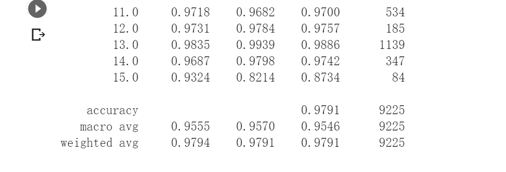
classification = classification_report(ytest, y_pred_test, digits=4)
print(classification)
在Hybrid中添加SENet
class HybridSN(nn.Module):

  def __init__(self):
    super(HybridSN, self).__init__()

    # 先做二维卷积
    self.conv1_2d = nn.Conv2d(30,64,(3,3))
    self.relu1 = nn.ReLU()
    # 3个三维卷积
    # conv2:(1, 30, 25, 25), 8个 7x3x3 的卷积核 ==> (8, 24, 23, 23)
    self.conv2_3d = nn.Conv3d(1, 8, kernel_size=(7, 3, 3), stride=1, padding=0)
    self.relu2 = nn.ReLU()
	# conv3:(8, 24, 23, 23), 16个 5x3x3 的卷积核 ==>(16, 20, 21, 21)
    self.conv3_3d = nn.Conv3d(8, 16, kernel_size=(5, 3, 3), stride=1, padding=0)
    self.relu3 = nn.ReLU()
	# conv4:(16, 20, 21, 21),32个 3x3x3 的卷积核 ==>(32, 18, 19, 19)
    self.conv4_3d = nn.Conv3d(16, 32, kernel_size=(3, 3, 3), stride=1, padding=0)
    self.relu4 = nn.ReLU()


	# 接下来依次为256,128节点的全连接层,都使用比例为0.4的 Dropout
    self.fn1 = nn.Linear(480896,256)
    self.fn2 = nn.Linear(256,128)
    self.fn3 = nn.Linear(128,16)
    self.drop = nn.Dropout(p = 0.4)


  def forward(self, x):
    # 先降到二维
    out = x.view(x.shape[0],x.shape[2],x.shape[3],x.shape[4])
    out = self.conv1_2d(out)
    # 升维(64, 23, 23)-->(1,64, 23, 23)
    out = out.view(out.shape[0],1,out.shape[1],out.shape[2],out.shape[3])

    out = self.conv2_3d(out)
    out = self.relu2(out)
    out = self.conv3_3d(out)
    out = self.relu3(out)
    out = self.conv4_3d(out)
    out = self.relu4(out)

    # 进行重组
    out = out.view(out.shape[0],-1)

    out = self.fn1(out)
    out = self.drop(out)
    out = self.fn2(out)
    out = self.drop(out)
    out = self.fn3(out)

    return outclass_num = 16

class HybridSN(nn.Module):

  def __init__(self):
    super(HybridSN, self).__init__()

    # 先做二维卷积
    self.conv1_2d = nn.Conv2d(30,64,(3,3))
    self.relu1 = nn.ReLU()
    # 3个三维卷积
    # conv2:(1, 30, 25, 25), 8个 7x3x3 的卷积核 ==> (8, 24, 23, 23)
    self.conv2_3d = nn.Conv3d(1, 8, kernel_size=(7, 3, 3), stride=1, padding=0)
    self.relu2 = nn.ReLU()
	# conv3:(8, 24, 23, 23), 16个 5x3x3 的卷积核 ==>(16, 20, 21, 21)
    self.conv3_3d = nn.Conv3d(8, 16, kernel_size=(5, 3, 3), stride=1, padding=0)
    self.relu3 = nn.ReLU()
	# conv4:(16, 20, 21, 21),32个 3x3x3 的卷积核 ==>(32, 18, 19, 19)
    self.conv4_3d = nn.Conv3d(16, 32, kernel_size=(3, 3, 3), stride=1, padding=0)
    self.relu4 = nn.ReLU()


	# 接下来依次为256,128节点的全连接层,都使用比例为0.4的 Dropout
    self.fn1 = nn.Linear(480896,256)
    self.fn2 = nn.Linear(256,128)
    self.fn3 = nn.Linear(128,16)
    self.drop = nn.Dropout(p = 0.4)


  def forward(self, x):
    # 先降到二维
    out = x.view(x.shape[0],x.shape[2],x.shape[3],x.shape[4])
    out = self.conv1_2d(out)
    # 升维(64, 23, 23)-->(1,64, 23, 23)
    out = out.view(out.shape[0],1,out.shape[1],out.shape[2],out.shape[3])

    out = self.conv2_3d(out)
    out = self.relu2(out)
    out = self.conv3_3d(out)
    out = self.relu3(out)
    out = self.conv4_3d(out)
    out = self.relu4(out)

    # 进行重组
    out = out.view(out.shape[0],-1)

    out = self.fn1(out)
    out = self.drop(out)
    out = self.fn2(out)
    out = self.drop(out)
    out = self.fn3(out)

    return out
class SELayer(nn.Module):
  def __init__(self,channel,r=16):
    super(SELayer,self).__init__()
    # 定义自适应平均池化函数,降采样
    self.avg_pool = nn.AdaptiveAvgPool2d(1)
    # 定义两个全连接层
    self.fc = nn.Sequential(
      nn.Linear(channel,round(channel/r)),
      nn.ReLU(inplace = True),
      nn.Linear(round(channel/r),channel),
      nn.Sigmoid()
    )

  def forward(self,x):
    b,c,_,_ = x.size()
    out = self.avg_pool(x).view(b,c)
    out = self.fc(out).view(b,c,1,1)
    out = x * out.expand_as(x)
    return out
class HybridSN(nn.Module):
  def __init__(self):
    super(HybridSN, self).__init__()
    self.conv3d_1 = nn.Sequential(
        nn.Conv3d(1, 8, kernel_size=(7, 3, 3), stride=1, padding=0),
        nn.BatchNorm3d(8),
        nn.ReLU(inplace = True),
    )
    self.conv3d_2 = nn.Sequential(
        nn.Conv3d(8, 16, kernel_size=(5, 3, 3), stride=1, padding=0),
        nn.BatchNorm3d(16),
        nn.ReLU(inplace = True),
    )
    self.conv3d_3 = nn.Sequential(
        nn.Conv3d(16, 32, kernel_size=(3, 3, 3), stride=1, padding=0),
        nn.BatchNorm3d(32),
        nn.ReLU(inplace = True)
    )

    self.conv2d_4 = nn.Sequential(
        nn.Conv2d(576, 64, kernel_size=(3, 3), stride=1, padding=0),
        nn.BatchNorm2d(64),
        nn.ReLU(inplace = True),
    )
    self.SElayer = SELayer(64,16)
    self.fc1 = nn.Linear(18496,256)
    self.fc2 = nn.Linear(256,128)
    self.fc3 = nn.Linear(128,16)
    self.dropout = nn.Dropout(p = 0.4)

  def forward(self,x):
    out = self.conv3d_1(x)
    out = self.conv3d_2(out)
    out = self.conv3d_3(out)
    out = self.conv2d_4(out.reshape(out.shape[0],-1,19,19))
    out = self.SElayer(out)
    out = out.reshape(out.shape[0],-1)
    out = F.relu(self.dropout(self.fc1(out)))
    out = F.relu(self.dropout(self.fc2(out)))
    out = self.fc3(out)
    return out
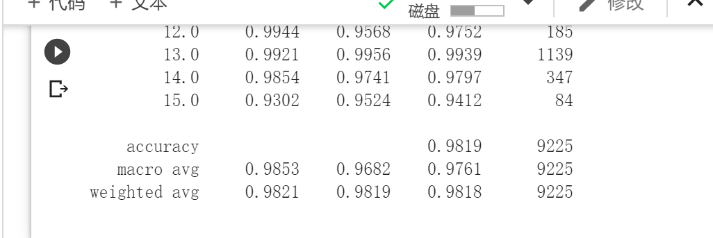
添加SENet模块后,模型的准确率有所提升,但是提升效果不明显。
《语义分割中的自注意力机制和低秩重建》
语义分割是将标签分配给图像中的像素的过程。这与分类形成了鲜明的对比,在分类中,一个标签被分配给整个图片。语义分割将同一类的多个对象视为一个实体。
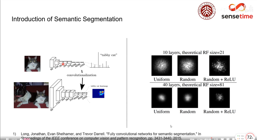
在《Fully convolutional networks for semantic segmentation》中提出了一种end-to-end的做semantic segmentation的方法,提出了全卷积网络的概念,将Alexnet这种的最后的全连接层转换为卷积层,好处就是可以输入任意的scale。只不过在输出的scale不同的时候,feature map的大小也不同,因为这里的目的是最piexl的语义分割,所以其实不重要。在Alexnet基础上, 最后的channel=4096的feature map经过一个1x1的卷积层, 变为channel=21的feature map, 然后经过上采样和crop, 变为与输入图像同样大小的channel=21的feature map, 也就是图中的pixel-wise prediction。 在Longjon的试验中一共有20个语义类别, 加上背景类别每个像素应该有21个softmax预测类, 因此pixel-wise prediction中channel=21。
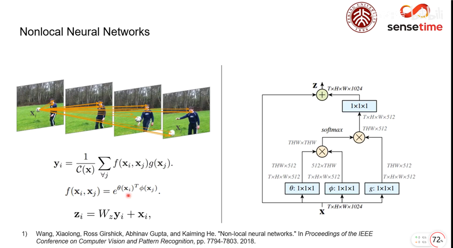
其中 ,
是像素个数,
是像素特征维度(通道数),
计算
和
之间的相关度(或称“能量”),
对
进行变换。可以看作对
的加权平均得到
,作为对
的重构,这里权重为
。
关于 和
的选择,作者列出了多个选项,并最终选择了
的形式,其中 分别对应 NLP Transformer 里的 query,key 和 value。此外,
经过
卷积后和
相加,作为 Non-local 模块的输出。最后结构图如下:
Non-local Block
其实,这里 和
的具体选择,对效果影响不大。这样计算出的
是个对称矩阵。甚至可以考虑将
转换省略,直接用
本身计算,而把
卷积放在模块之前之后,这样的效果也不逊色。
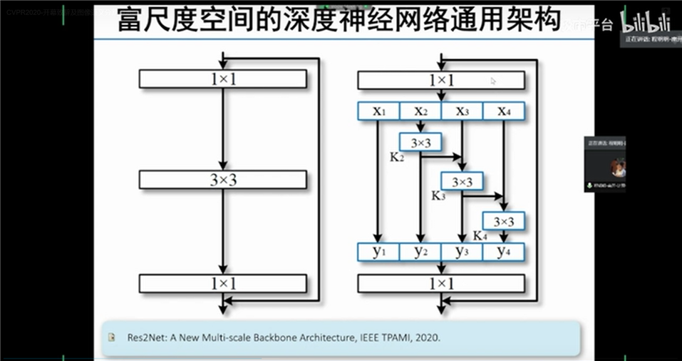
《图像语义分割前沿进展》
富尺度空间的深度神经网络通用架构Res2Net和其应用场景以及自适应的池化方式Strip Pooling。
基于条带池化,我们深入了解了空间池化的架构设计:(1)引入了新的条带池化模型,可以使主干网络可以有效地捕捉长距离的依赖关系;(2)提出了一个新颖的、可以将不同的空间池化作为核心的构件块;(3)有组织地在性能上比较了所提出的条带池化和传统的空间池化技术的差别。
平均值池化操作:
Standard Spatial Average Pooling:记输入的二维张量为 ,尺寸为
。在平均值池化层中,需要池化的空间范围
。因此,输出的二维张量
,尺寸为
。平均值池化的过程可以表示为:
其中,
,每一个
的位置都对应于一个
的窗口。上述池化操作已成功应用于收集远程上下文的先前工作。但是,在处理形状不规则的物体时,可能会不可避免地合并许多不相关的区域。
Strip Pooling:为了缓解上述问题,我们在这里提出“条带池化”的概念,它使用带状池化窗口沿着水平或垂直维度执行池化。在数学上,记输入的二维张量为 ,尺寸为
,在条带池化中,池化窗口为
或
。与二维平均值池化不同的是,条带池化对行或列中的所有特征值进行平均。其表达式为:
给定水平和垂直条带池化层,由于长而窄的核形状,很容易在离散分布的区域之间建立远程依赖关系,并对带状形状的区域进行编码。同时,由于其沿其他维度的窄核形状,它还专注于捕获局部细节。这些特性使提出的条带池化与依赖于方形内核的常规空间池化不同。
标签:axis fse 方式 oss conv2 选项 scale 场景 对比
原文地址:https://www.cnblogs.com/Dingding03/p/13510061.html