标签：holo   The   method   via   cti   transform   simple   ntile   oba   

Introduction

This article is about some concepts of the biomedical data analysis.

Question 1

(a) First-principle(FP) models & Data driven(DD) models

Defination/Difference:

• FP models: it‘s a analytical modeling, based on a basic model originating from mathematical relations derived from the first-principle equations and use understanding of the system underlying physics to derive its mathematical representation.
• DD models: Use system test data to derive its mathmatical representation.

Disadvantages and Advantages:

• FP models: Have a good insight into the mechanism of the system but it‘s difficult to match data and determine the phenomenological parameters.
• DD models: the advantage is the speed in which an accurate model can be constructed and confidence gained thanks to the use of the data obtained from the actual system but it‘s less interpretable and need to handle multiple data sets in order to cover the range of system operation.

(b)&(c) Normal Probability Distribution

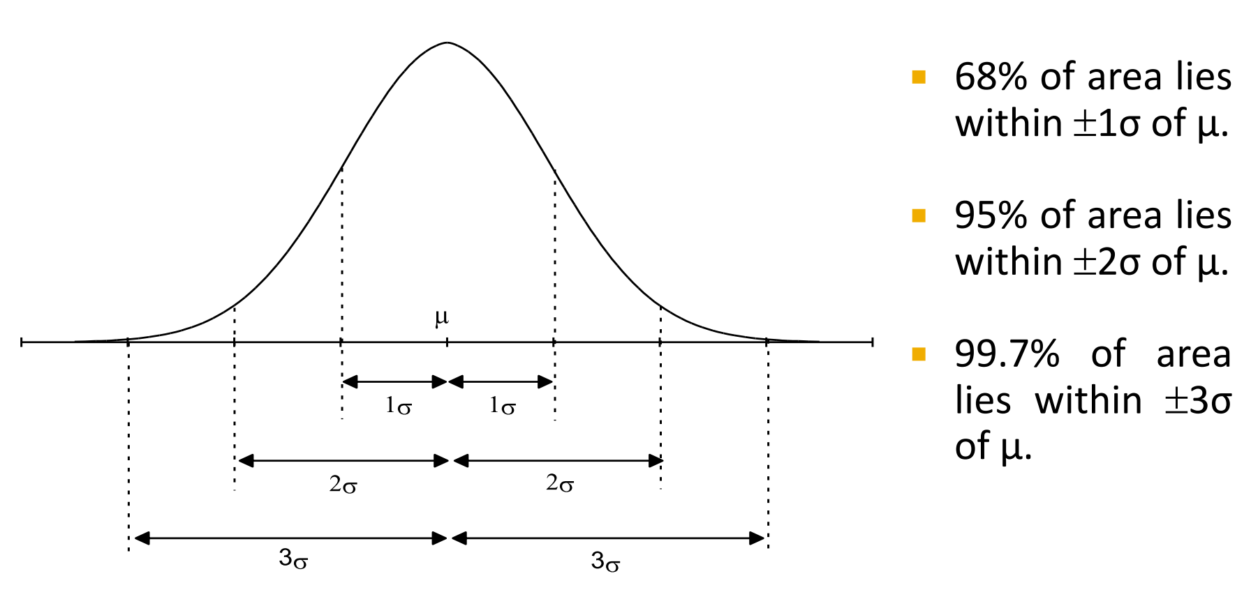
Plot: the normal probability distribution clearly marking the mean, standard deviation,
and the percentage of data contained within one, two, and three standard deviations
around the mean.

Computation:
the median, interquartile range, and the value that corresponds to the 5th percentile.(mean=50000,sd=7000)

(d) Correlation & Dependence

Understand in statistical sense: correlation or dependence any statistical relationship between two random variables. They measure how two variables X, y co-vary.

Difference:
The correlation commonly refers to the degree to which a pair of variables are linearly related. So, if correlation cofficients are 0, it not means that a pair of variables are independent unless they don‘t have nonlinear relationship. Fomally, random variables are dependent if they do not satisfy a mathmatical property of probabilitic independence.

Measurement:

• Correlation based approaches: Capture only linear (or at least only monotonic) statistical relationships.
• Probability density based approaches: Divergence metrics (e.g. mutual information)

(e) Data Sampling and Collection

Key question in sampling:

• Sample rate: determine the frequency of measurement.
• Sample size: study population.
• Segment: select signal segment in time series.

empirical rule of sampling data:

• Sample size: At least 25-30 samples per category in the data and larger sample size means greater statistical power.
• Equipment: Err on the side of larger sample rate and Test equipment on pilot data
• Data source: Ensure your data is as representative as possible and Use additional external datasets, when possible.

(f) Fourier transform

Reasons of use:

• Signal data: complex
• Fourier transform: decompose the signal into its constituent frequencies.(Describe the time series referring to different properties)

Underlying Philosophy:
From time domain analysis to frequency domain analysis. Describe one onject referring to different properties.

Assumption:
Express a signal as an infinite sum of sinusoids and requires uniformly sampled data.

Examples with Plot:

Key Limitation:

• Sample Size: more samples means more statistic power
• Limitation: A limitation of the Fourier transform is that it‘s not truly realizable in practice - we can never sample a function for every \(X\in R\) This can be mitigated by the way we do integrals numerically: we do Riemann sums, which naturally require sampling your function anyway! So we might not get the true Fourier transform of a recorded sound for instance but we can get pretty close!

Question 2

(a)Kernel density estimation

How it works:
Add noise to each observation (impose a kernel, typically Gaussian kernel)

whereK \(\mathcal{K}\) is the kernel — a non-negative function — and h > 0 is a smoothing parameter called the bandwidth.

type of variables:
Continuous variables

Comment on bandwidth:
The bandwidth of the kernel is a free parameter which exhibits a strong influence on the resulting estimate. If the bandwidth is too small, the density curve may become undersmoothed and overfitted but if it is too large, the density curve will become oversmoothed, leading to the terrible estimation of the density.

(b)p-value

p-value defination:
it can be interpreted as the probability of obtaining a similar result by chance if the null hypothesis is true. It also measure the probability of the occurance of extreme samples.

key pitfalls:
p-value is just Confirmatory data analysis. Using it, we just can accept or reject the null hypothesis but in case we get the result that we reject the null hypothesis, we can not claim that we accept the alternative hypothesis.

Assess two variables:
Use Kolmogorov-Smirnov test to(or Wilcoxn test) compare if the statistical properties of two variables are the same.

p-hacking:
P-hacking refers to the practice of reanalyzing data in many different ways to yield a target result. They, and more recently Motulsky, have described the variations on P-hacking, and the hazards, notably the likelihood of false positives—findings that statistics suggest are meaningful when they are no.

(c)Central moment

Generalization:
a central moment is a moment of a probability distribution of a random variable about the random variable‘s mean; that is, it is the expected value of a specified integer power of the deviation of the random variable from the mean.

We can extend the concept of the quantifying statistical relationships beyond the two central order moments.

If m is even, the possible value should greater than 0.

(d) Sparsity

Description:
A sparse matrix, intuitively, is a matrix in which most of the elements are 0. The number of zero-valued elements divided by the total number of elements (e.g., m × n for an m × n matrix) is sometimes referred to as the sparsity of the matrix.

principle of parsimony:
The principle that the most acceptable explanation of an occurrence, phenomenon, or event is the simplest, involving the fewest entities, assumptions, or changes.

Examples:
The principle of parsimony can be seen in many feature selection methods like Lasso regression, if the dimension of the data is too large, lasso is a good way to press the unimportant variables to 0, get the important features and reduce the dimension eventually.

Benefits:

• Sometimes the simpler explanation are more likely to be true.
• Many biostatistics problems (like gene problems) have very high dimensions. Some general methods (such as SVM) are difficult to apply to highdimensional data, so it is necessary to reduce the dimension to deal with them.
• There are many redundant variables that are invalid to analyze problems. Deleting them will save time and improve efficiency

(e) Feature selection & Feature transformation

Feature transformation:
Construct lower dimensional space where the new data points retain the distance of the data points in the original feature space (PCA; Factor analyse).

Feature selection:
Discard non-contributing features towards predicting the outcome. (Lasso; Forward subset selection)

Difference:
Feature transformation maps the original variable space to a low dimensional space, and realizes dimension reduction. In this process, new variables are generated (principle components or factors). However, feature selection is to select the important variables from the original variables, and get a subset of the original variables, which does not produce new variables in the process.

Advantages:

• Feature selection:
  • Interpretable
  • retain domain expertise
  • often is the only useful approach in practice
  • Saves on resources on data collection or data processing
• Feature transformation
  • Variable transformation produces new variables, which can find new connections between variables (principle component), or potential factor within variables, so it can provide new ideas and directions for analysis.

Preference:
feature selection is the preference in the analysis of biomedical data applications because of its interpretation while feature transform will create new variable which we can not interprete well. Reliable transformation in high dimensional spaces is problematic, and it does not save up on resources on data collection or data processing.

(f) Confusion matrix

Definetion:
Confusion matrix is a specific table layout that allows visualization of the performance of an algorithm. Each row of the matrix represents the instances in a predicted class, while each column represents the instances in an actual class. Therefore, the matrix makes it easy to see whether the system is confusing two classes.

Application:
In claasification problems, confusion matrix can be used to assess our mapping model. Through it, we can calculate its sensitivity, specificity, precision and recall which is used to check the accurancies of our results.

Examples:
a dataset which relates to subarachnoid hemorrhage (SAH). SAH is a rare, potentially fatal, type of stroke caused by bleeding on the surface of the brain. Now, we have fitted a simple model containing only age and gender, and the assessed results of patients are recorded in outcome variable. This model is a logistic model:

Then, we can use this model to prediction our dataset and using those predictions and true value, we can draw the confusion table to evaluation the capabilities of this logistic model.

Question 3

(a)generic methodology

If y is catigorical and discrete variable, then we say this is a classification problem. For this, the generic methodologies are logistic regression(LR), KNN, SVM, Random forest(RF)..

If y is continuous variable, and this is a regression problem, the generic methologies are Ordinary Least Squares (OLS) regression (linear regression), Support Vector Machines (SVM), Random Forests (RF)

Example: We use a dataset which relates to subarachnoid hemorrhage (SAH). There are 113 observations and we use gender and age to predict the outcom. In this problem the size of X is (113,2) and the size of the outcome is (113,1)

(b) Correlation coefficients

Definetion:
Linear correlation coefficient is a statistics to measure the degree of linear correlation between two variables, it can be calculated as:

Range:
correlation coeffiients are in the interval [-1,1].

Interpretation: Measure the co-variance of the X and Y. If they have linear relationship, we can find that:

On contrast, if they are independent, the correlation coefficients are near to 0. However, this coefficient just can reflect the linear relationship.

Reliable: When the correlation coefficients are approach to 1 or -1, in other words, the coefficients are far from 0, I believe the relationship is statistically strong.

Correlation matrix:
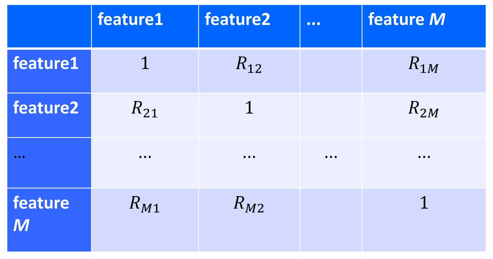
It can indicate there is a strong correlation between i and j variables if (i, j) element in correlation matrix is large

(c) Regression and Classification

Regression and Classification:
First of all, our dataset need contain design matrix X and reponse y.

• Classification: y is discrete and catigorical vaeiable. And what we learn is \(f(X)=y:classifier\). The indicative algorithmic approaches of this type of problems have: KNN,LR,SVM,RF
• Regression: y is cntimuouse variable and regressors. The learner is \(f(X)=y:regressor\). The indicative algorithmic approaches of this type of problems have: OLS,SVM,RF

(d) Linear Regression

Computation:

• intercept:

• Linear regression coefficients:

Of course, we can use matrix method to deduct these results to calculate the coefficients and intercept.

Indicators for good linear regression:

• Mean square error is small.
• R2 is close to 1.
• The QQ-plot of residuals are on the same line.
• There is no obvious trend in residual plot.

Residuals:
If there is a pattern in the residuals, it means that residuals are related to y or other residuals,

• you might need to add the higher order term of X
• change the form of X (like log(X)).
• Add new explanatory variables.

(e) Model validation

Generic method:
Cross validation method.First, Randomly split the data in design matrix X into 10 groups with same size. Then sequentially regard 9 groups of them as training data, and one for testing. Repeat process 10 iterations, each time randomly splitting dataset.

Performance:
For classification problem, we can print out confusion matrix, and for regression problem, we can calculate MSE (mean squared error). If we want to compromise between performance and complexity, we can also calculate AIC or BIC statistics.

Present result:

• Report metrics on testing data (out-of-sample dataset).
• ROC curve and AUC value.

(f)&(g) Linear regression summary

linear least squares regression model:

Significant variables:
ADV, R1 and R2 are statistically significant

Goodness
Yes, It is a good statistics mapping model because the \(R^2 = 0.956\) and \(adjusted\ R^2 = 0.941\), very close to 1, which means that the model fit well.

Performance with new data
If I had resources to collect the new data, I will apply this model to new data to
get the predictive ?y, compare it with observed data, calculate the MSE. The MSE in the test set can better reflect the generalization ability of the model.

(h) Logistic regression

If the p calculated by the above equation is more than 0.5, the patient can be discharged from the hospital. If it is less than 0.5, the patient can not be discharged. If the BT = 29, then the\(p = \frac{1}{1+e^{-(60-2*29)}}=0.881\), the patient can be discharged from the hospital

2021-4-23 BioDSTest2019

标签：holo   The   method   via   cti   transform   simple   ntile   oba   

原文地址：https://www.cnblogs.com/DS-blog-HWH/p/14702668.html