标签:
PMF
A discrete random variable $X$ is said to have a Poisson distribution with parameter $\lambda > 0$, if the probability mass function of $X$ is given by $$f(x; \lambda) = \Pr(X=x) = e^{-\lambda}{\lambda^x\over x!}$$ for $x=0, 1, 2, \cdots$.
Proof:
$$ \begin{align*} \sum_{x=0}^{\infty}f(x; \lambda) &= \sum_{x=0}^{\infty} e^{-\lambda}{\lambda^x\over x!}\\ & = e^{-\lambda}\sum_{x=0}^{\infty}{\lambda^x\over x!}\\ &= e^{-\lambda}\left(1 + \lambda + {\lambda^2 \over 2!}+ {\lambda^3\over 3!}+ \cdots\right)\\ & = e^{-\lambda} \cdot e^{\lambda}\\ & = 1 \end{align*} $$
Mean
The expected value is $$\mu = E[X] = \lambda$$
Proof:
$$ \begin{align*} E[X] &= \sum_{x=0}^{\infty}xe^{-\lambda}{\lambda^x\over x!}\\ & = \sum_{x=1}^{\infty}e^{-\lambda}{\lambda^x\over (x-1)!}\\ & =\lambda e^{-\lambda}\sum_{x=1}^{\infty}{\lambda^{x-1}\over (x-1)!}\\ & = \lambda e^{-\lambda}\left(1+\lambda + {\lambda^2\over 2!} + {\lambda^3\over 3!}+\cdots\right)\\ & = \lambda e^{-\lambda} e^{\lambda}\\ & = \lambda \end{align*} $$
Variance
The variance is $$\sigma^2 = \mbox{Var}(X) = \lambda$$
Proof:
$$ \begin{align*} E\left[X^2\right] &= \sum_{x=0}^{\infty}x^2e^{-\lambda}{\lambda^x\over x!}\\ &= \sum_{x=1}^{\infty}xe^{-\lambda}{\lambda^x\over (x-1)!}\\ &= \lambda\sum_{x=1}^{\infty}xe^{-\lambda}{\lambda^{x-1}\over (x-1)!}\\ & = \lambda\sum_{x=1}^{\infty}(x-1+1)e^{-\lambda}{\lambda^{x-1}\over (x-1)!}\\ &= \lambda\left(\sum_{x=1}^{\infty}(x-1)e^{-\lambda}{\lambda^{x-1}\over (x-1)!} + \sum_{x=1}^{\infty} e^{-\lambda}{\lambda^{x-1}\over (x-1)!}\right)\\ &= \lambda\left(\lambda\sum_{x=2}^{\infty}e^{-\lambda}{\lambda^{x-2}\over (x-2)!} + \sum_{x=1}^{\infty} e^{-\lambda}{\lambda^{x-1}\over (x-1)!}\right)\\ & = \lambda(\lambda+1) \end{align*} $$ Hence the variance is $$ \begin{align*} \mbox{Var}(X)& = E\left[X^2\right] - E[X]^2\\ & = \lambda(\lambda + 1) - \lambda^2\\ & = \lambda \end{align*} $$
Examples
1. Let $X$ be Poisson distributed with intensity $\lambda=10$. Determine the expected value $\mu$, the standard deviation $\sigma$, and the probability $P\left(|X-\mu| \geq 2\sigma\right)$. Compare with Chebyshev‘s Inequality.
Solution:
The Poisson distribution mass function is $$f(x) = e^{-\lambda}{\lambda^x\over x!},\ x=0, 1, 2, \cdots$$ The expected value is $$\mu= \lambda=10$$ Then the standard deviation is $$\sigma = \sqrt{\lambda} = 3.162278$$ The probability that $X$ takes a value more than two standard deviations from $\mu$ is $$ \begin{align*} P\left(|X-\lambda| \geq 2\sqrt{\lambda}\right) &= P\left(X \leq \lambda-2\sqrt{\lambda}\right) + P\left(X \geq \lambda + 2\sqrt{\lambda}\right)\\ & = P(X \leq 3) + P(X \geq 17)\\ & = 0.03737766 \end{align*} $$ R code:
sum(dpois(c(0:3), 10)) + 1 - sum(dpois(c(0:16), 10))
# [1] 0.03737766
Chebyshev‘s Inequality gives the weaker estimation $$P\left(|X - \mu| \geq 2\sigma\right) \leq {1\over2^2} = 0.25$$
2. In a certain shop, an average of ten customers enter per hour. What is the probability $P$ that at most eight customers enter during a given hour.
Solution:
Recall that the Poisson distribution mass function is $$P(X=x) = e^{-\lambda}{\lambda^x\over x!}$$ and $\lambda=10$. So we have $$ \begin{align*} P(X \leq 8) &= \sum_{x=0}^{8}e^{-10}{10^{x}\over x!}\\ &= 0.3328197 \end{align*} $$ R code:
sum(dpois(c(0:8), 10))
# [1] 0.3328197
ppois(8, 10)
# [1] 0.3328197
3. What is the probability $Q$ that at most 80 customers enter the shop from the previous problem during a day of 10 hours?
Solution:
The number $Y$ of customers during an entire day is the sum of ten independent Poisson distribution with parameter $\lambda=10$. $$Y = X_1 + \cdots + X_{10}$$ Thus $Y$ is also a Poisson distribution with parameter $\lambda = 100$. Thus we have $$ \begin{align*} P(Y \leq 80) &= \sum_{y=0}^{80}e^{-100}{100^{y}\over y!}\\ &= 0.02264918 \end{align*} $$ R code:
sum(dpois(c(0:80), 100))
# [1] 0.02264918
ppois(80, 100)
# [1] 0.02264918
Alternatively, we can use normal approximation (generally when $\lambda > 9$) with $\mu = \lambda = 100$ and $\sigma = \sqrt{\lambda}=10$. $$ \begin{align*} P(Y \leq 80) &= \Phi\left({80.5-100\over 10 }\right)\\ &= \Phi\left({-19.5\over10}\right)\\ &=0.02558806 \end{align*} $$ R code:
pnorm(-19.5/10)
# [1] 0.02558806
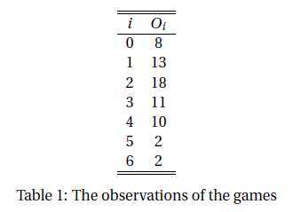
4. At the 2006 FIFA World Championship, a total of 64 games were played. The number of goals per game was distributed as follows: 8 games with 0 goals 13 games with 1 goal 18 games with 2 goals 11 games with 3 goals 10 games with 4 goals 2 games with 5 goals 2 games with 6 goals Determine whether the number of goals per game may be assumed to be Poisson distributed.
Solution:
We can use Chi-squared test. The observations are in Table 1.
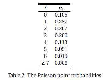
On the other hand, if this is a Poisson distribution then the parameter should be $$ \begin{align*} \lambda &= \mu\\ & = {0\times8 + 1\times13 +\cdots + 6\times2 \over 8+13+\cdots+2}\\ & = {144\over 64}\\ &=2.25 \end{align*} $$ And the Poisson point probabilities are listed in Table 2.
And hence the expected numbers are listed in Table 3.
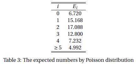
Note that we have merged some categories in order to get $E_i \geq 3$. The statistic is $$ \begin{align*} \chi^2 &= \sum{(O-E)^2\over E}\\ &= {(8-6.720)^2 \over 6.720} + \cdots + {(4-4.992)^2 \over 4.992}\\ &= 2.112048 \end{align*} $$ There are six categories and thus the degree of freedom is $6-1 = 5$. The significance probability is 0.8334339. R code:
prob = c(round(dpois(c(0:6), 2.25), 3),
+          1 - round(sum(dpois(c(0:6), 2.25)), 3))
expect = prob * 64
prob; expect
# [1] 0.105 0.237 0.267 0.200 0.113 0.051 0.019 0.008
# [1]  6.720 15.168 17.088 12.800  7.232  3.264  1.216  0.512
O = c(8, 13, 18, 11, 10, 4)
E = c(expect[1:5], sum(expect[6:8]))
O; E
# [1]  8 13 18 11 10  4
# [1]  6.720 15.168 17.088 12.800  7.232  4.992
chisq = sum((O - E) ^ 2 / E)
1 - pchisq(chisq, 5)
# [1] 0.8334339
The hypothesis is $$H_0: \mbox{Poisson distribution},\ H_1: \mbox{Not Poisson distribution}$$ Since $p = 0.8334339 > 0.05$, so we accept $H_0$. That is, it is reasonable to claim that the number of goals per game is Poisson distributed.
Reference
基本概率分布Basic Concept of Probability Distributions 2: Poisson Distribution
标签:
原文地址:http://www.cnblogs.com/zhaoyin/p/4199022.html