标签:
In?statistics, the?bias?(or?bias function) of an?estimator?is the difference between this estimator‘s?expected value?and the true value of the parameter being estimated. An estimator or decision rule with zero bias is called?unbiased. Otherwise the estimator is said to be?biased. In statistics, "bias" is an objective statement about a function, and while not a desired property, it is not pejorative, unlike the ordinary English use of the term "bias".
All else equal, an unbiased estimator is preferable to a biased estimator, but in practice all else is not equal, and biased estimators are frequently used, generally with small bias. When a biased estimator is used, the bias is also estimated. A biased estimator may be used for various reasons: because an unbiased estimator does not exist without further assumptions about a population or is difficult to compute (as in?unbiased estimation of standard deviation); because an estimator is median-unbiased but not mean-unbiased (or the reverse); because a biased estimator reduces some?loss function?(particularly?mean squared error) compared with unbiased estimators (notably in?shrinkage estimators); or because in some cases being unbiased is too strong a condition, and the only unbiased estimators are not useful. Further, mean-unbiasedness is not preserved under non-linear transformations, though median-unbiasedness is (see?effect of transformations); for example, the?sample variance?is an unbiased estimator for the population variance, but its square root, the?sample standard deviation, is a biased estimator for the population standard deviation. These are all illustrated below.
Suppose we have a?statistical model, parameterized by a real number? , giving rise to a probability distribution for observed data,?
 , and a statistic?
 which serves as an?estimator?of?
 ?based on any observed data?
 . That is, we assume that our data follows some unknown distribution?
 ?(where?
 ?is a fixed constant that is part of this distribution, but is unknown), and then we construct some estimator?
 ?that maps observed data to values that we hope are close to?
 . Then the?bias?of this estimator (relative to the parameter?
 ) is defined to be
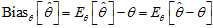
where? denotes?expected value?over the distribution?
 , i.e. averaging over all possible observations?
 . The second equation follows since?
 ?is measurable with respect to the conditional distribution?
 .
.
An estimator is said to be?unbiased?if its bias is equal to zero for all values of parameter? .
.
There are more general notions of bias and unbiasedness. What this article calls "bias" is called "mean-bias", to distinguish?mean-bias from the other notions, with the notable ones being "median-unbiased" estimators. For more details, the general theory of unbiased estimators is briefly discussed near the end of this article.
This article uses the following symbols and definitions:
 ?is the population mean
 is the sample mean
 is the population variance
 is the biased sample variance (i.e. without Bessel‘s correction)
 is the unbiased sample variance (i.e. with Bessel‘s correction)
The standard deviations will then be the square roots of the respective variances. Since the square root introduces bias, the terminology "uncorrected" and "corrected" is preferred for the standard deviation estimators:
 is the uncorrected sample standard deviation (i.e. without Bessel‘s correction)
 ?is the corrected sample standard deviation (i.e. with Bessel‘s correction), which is less biased, but still biased
In general, the?population variance?of a?finite?population?of size? ?with values?
 is given by

Where

is the population mean. The population variance therefore is the variance of the underlying probability distribution. In this sense, the concept of population can be extended to continuous random variables with infinite populations.
In many practical situations, the true variance of a population is not known?a priori?and must be computed somehow. When dealing with extremely large populations, it is not possible to count every object in the population, so the computation must be performed on a?sample?of the population.[7]?Sample variance can also be applied to the estimation of the variance of a continuous distribution from a sample of that distribution.
The?sample variance?of a random variable demonstrates two aspects of estimator bias: firstly, the naive estimator is biased, which can be corrected by a scale factor; second, the unbiased estimator is not optimal in terms of?mean squared error?(MSE), which can be minimized by using a different scale factor, resulting in a biased estimator with lower MSE than the unbiased estimator. Concretely, the naive estimator sums the squared deviations and divides by?n,?which is biased. Dividing instead by?n???1 yields an unbiased estimator. Conversely, MSE can be minimized by dividing by a different number (depending on distribution), but this results in a biased estimator. This number is always larger than?n???1, so this is known as a?shrinkage estimator, as it "shrinks" the unbiased estimator towards zero; for the normal distribution the optimal value is?n?+?1.
Suppose we take a?sample with replacement?of?n?values? from the population(with?expectation?
 ?and?variance?
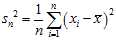
 ), where?n?<?N, and estimate the variance on the basis of this sample. If the?sample mean?and uncorrected?sample variance?are defined as
 ,
, 
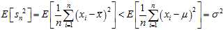
then? is a biased estimator of?
 , because
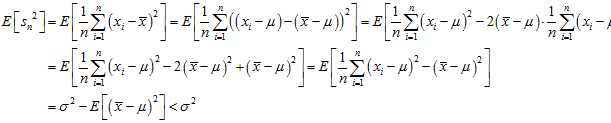
In other words, the expected value of the uncorrected sample variance does not equal the population variance? , unless multiplied by a normalization factor. The sample mean, on the other hand, is an unbiased?estimator of the population mean?
 .
.
The reason that? ?is biased stems from the fact that the sample mean is an?ordinary least squares?(OLS) estimator for?
 :?
:? ?is the number that makes the sum?
 ?as small as possible. That is, when any other number is plugged into this sum, the sum can only increase. In particular, the choice?
 ?gives,
and then
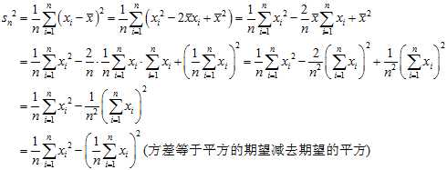
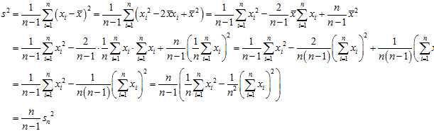
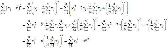
Note that the usual definition of sample variance is
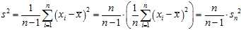
and this is an unbiased estimator of the population variance. This can be seen by noting the following formula, which follows from the?Bienaymé formula, for the term in the inequality for the expectation of the uncorrected sample variance above:
The ratio  between the biased (uncorrected) and unbiased estimates of the variance is known as?Bessel‘s correction.
Suppose the mean of the whole population is 2050, but the statistician does not know that, and must estimate it based on this small sample chosen randomly from the population:
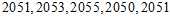
One may compute the sample average:
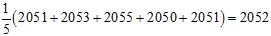
This may serve as an observable estimate of the unobservable population average, which is?2050. Now we face the problem of estimating the population variance. That is the average of the squares of the deviations from?2050. If we knew that the population average is 2050, we could proceed as follows:

But our estimate of the population average is the sample average,?2052, not?2050. Therefore we do what we can:

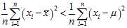
This is a substantially smaller estimate. Now a question arises: is the estimate of the population variance that arises in this way using the sample mean?always?smaller than what we would get if we used the population mean? The answer is?yes?except when the sample mean happens to be the same as the population mean.
We are seeking the sum of squared distances from the population mean, but end up calculating the sum of squared differences from the sample mean, which, as will be seen, is the number that minimizes that sum of squared distances. So unless the sample happens to have the same mean as the population, this estimate will always underestimate the population variance.
To see why this happens, we use a simple identity in algebra:
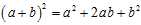
With  ?representing the deviation from an individual to the sample mean, and
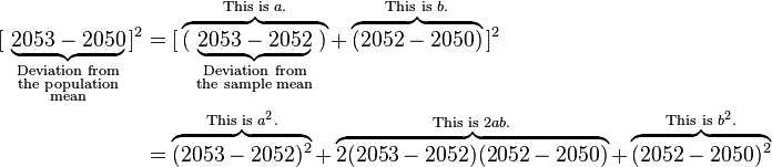
  ?representing the deviation from the sample mean to the population mean. Note that we‘ve simply decomposed the actual deviation from the (unknown) population mean into two components: the deviation to the sample mean, which we can compute, and the additional deviation to the population mean, which we can not. Now apply that identity to the squares of deviations from the population mean:
Now apply this to all five observations and observe certain patterns:
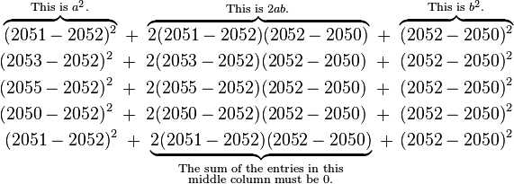
The sum of the entries in the middle column must be zero because the sum of the deviations from the sample average must be zero. When the middle column has vanished, we then observe that
 ) is the sum of the squares of the deviations from the sample mean;
 ?and?
?and? ) is the sum of squares of the deviations from the population mean, because of the way we started with?[2053???2050]2, and did the same with the other four entries;
Therefore:
That is why the sum of squares of the deviations from the?sample?mean is too small to give an unbiased estimate of the population variance when the average of those squares is found.
In?statistics,?Bessel‘s correction, named after?Friedrich Bessel, is the use of  instead of
  ?in the formula for the?sample variance?and?sample standard deviation, where?
 ?is the number of observations in a sample. This corrects the bias in the estimation of the population variance, and some (but not all) of the bias in the estimation of the population standard deviation, but often increases the?mean squared error?in these estimations.
That is, when?estimating?the population?variance?and?standard deviation?from a sample when the population mean is unknown, the sample variance estimated as the?mean?of the squared deviations of sample values from their mean (that is, using a multiplicative factor? ) is a?biased estimator?of the population variance, and for the average sample underestimates it. Multiplying the standard sample variance as computed in that fashion by?
 (equivalently, using?
 instead of?
 in the estimator‘s formula) corrects for this, and gives an unbiased estimator of the population variance. In some terminology, the factor?
 is itself called?Bessel‘s correction.
One can understand Bessel‘s correction intuitively as the?degrees of freedom?in the?residuals?vector (residuals, not errors, because the population mean is unknown):
where? ?is the sample mean. While there are?
 independent samples, there are only?
 independent residuals, as they sum to 0.
Three caveats must be borne in mind regarding Bessel‘s correction: firstly, it does not yield an unbiased estimator of standard?deviation;?secondly, the corrected estimator often has worse (higher)?mean squared error?(MSE) than the uncorrected estimator, and never has the minimum MSE: a different scale factor can always be chosen to minimize MSE; thirdly it is only necessary when the population mean is unknown (and estimated as the sample mean).
The first is a subtle point: while the sample variance (using Bessel‘s correction) is an unbiased estimate of the population variance, its?square root, the sample standard deviation, is a?biased?estimate of the population standard deviation; because the square root is a?concave function, the bias is downward, by?Jensen‘s inequality. There is no general formula for an unbiased estimator of the population standard deviation, though there are correction factors for particular distributions, such as the normal; seeunbiased estimation of standard deviation?for details. An approximation for the exact correction factor for the normal distribution is given by using?n???1.5 in the formula: the bias decays quadratically (rather than linearly, as in the uncorrected form and Bessel‘s corrected form).
Secondly, the unbiased estimator does not minimize MSE compared with biased estimators, and generally has worse MSE than the uncorrected estimator (this varies with?excess kurtosis). MSE can be minimized by using a different factor. The optimal value depends on excess kurtosis, as discussed in?mean squared error: variance; for the normal distribution this is optimized by dividing by?n?+?1 (instead of?n???1 or?n).
Thirdly, Bessel‘s correction is only necessary when the population mean is unknown, and one is estimating?both?population mean?and?population variance from a given sample set, using the sample mean to estimate the population mean. In that case there aren?degrees of freedom in a sample of?n?points, and simultaneous estimation of mean and variance means one degree of freedom goes to the sample mean and the remaining?n???1 degrees of freedom (the?residuals) go to the sample variance. However, if the population mean is known, then the deviations of the samples from the population mean have?n?degrees of freedom (because the mean is not being estimated – the deviations are not residuals but?errors) and Bessel‘s correction is not applicable.
This correction is so common that the term "sample variation" and "sample standard deviation" are frequently used to mean the corrected estimators (unbiased sample variation, less biased sample standard deviation), using? . However caution is needed: some calculators and software packages may provide for both or only the more unusual formulation.
The sample mean is given by

The biased sample variance is then written:
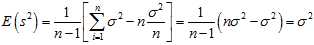
and the unbiased sample variance is written:
As a background fact, we use the identity?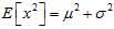 ?which follows from the definition of the standard deviation and?linearity of expectation.
A very helpful observation is that for any distribution, the variance equals half the expected value of? ?when?
 ?are independent samples. To prove this observation we will use that?
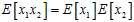 ?(which follows from the fact that they are independent) as well as linearity of expectation:

Now that the observation is proven, it suffices to show that the expected squared difference of two samples from the sample population? ?equals?
 ?times the expected squared difference of two samples from the original distribution. To see this, note that when we pick?
 ?and?
?and? ?via?
?via? ?being integers selected independently and uniformly from 1 to?
 , a fraction?
 ?of the time we will have?
 ?and therefore the sampled squared difference is zero independent of the original distribution. The remaining?
 ?of the time, the value of?
 ?is the expected squared difference between two unrelated samples from the original distribution. Therefore, dividing the sample expected squared difference by?
 , or equivalently multiplying by?
 gives an unbiased estimate of the original expected squared difference.
Recycling an?identity for variance,
So

and by definition,

Note that, since? ?are a random sample from a distribution with variance?
 , it follows that for each?
 :
:

and also

This is a property of the variance of uncorrelated variables, arising from the?Bienaymé formula. The required result is then obtained by substituting these two formulae:
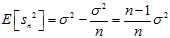
The expected discrepancy between the biased estimator and the true variance is
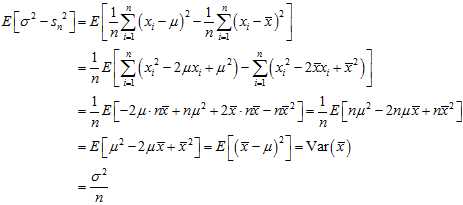
So, the expected value of the biased estimator will be
So, an unbiased estimator should be given by

In the biased estimator, by using the sample mean instead of the true mean, you are underestimating each? ?by?
?by? . We know that the variance of a sum is the sum of the variances (for uncorrelated variables). So, to find the discrepancy between the biased estimator and the true variance, we just need to find the variance of?
 .
.
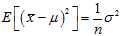
This is just the?variance of the sample mean, which is? . So, we expect that the biased estimator underestimates?
 ?by?
?by? , and so the biased estimator = (1???1/n)?×?the unbiased estimator = (n???1)/n?×?the unbiased estimator.
标签:
原文地址:http://www.cnblogs.com/yiyuehuan/p/4574303.html